Data Visualization
Contents
Data Visualization
In this notebook, we conduct data visulization on the clean data.
Load the data
import numpy as np
import pandas as pd
import matplotlib.pyplot as plt

clean_data = pd.read_csv("../data/clean.csv")
clean_data.head()
| id | diagnosis | radius_mean | texture_mean | perimeter_mean | area_mean | smoothness_mean | compactness_mean | concavity_mean | concave points_mean | ... | radius_worst | texture_worst | perimeter_worst | area_worst | smoothness_worst | compactness_worst | concavity_worst | concave points_worst | symmetry_worst | fractal_dimension_worst | |
|---|---|---|---|---|---|---|---|---|---|---|---|---|---|---|---|---|---|---|---|---|---|
| 0 | 842302 | 1.0 | 17.99 | 10.38 | 122.80 | 1001.0 | 0.11840 | 0.27760 | 0.3001 | 0.14710 | ... | 25.38 | 17.33 | 184.60 | 2019.0 | 0.1622 | 0.6656 | 0.7119 | 0.2654 | 0.4601 | 0.11890 |
| 1 | 842517 | 1.0 | 20.57 | 17.77 | 132.90 | 1326.0 | 0.08474 | 0.07864 | 0.0869 | 0.07017 | ... | 24.99 | 23.41 | 158.80 | 1956.0 | 0.1238 | 0.1866 | 0.2416 | 0.1860 | 0.2750 | 0.08902 |
| 2 | 84300903 | 1.0 | 19.69 | 21.25 | 130.00 | 1203.0 | 0.10960 | 0.15990 | 0.1974 | 0.12790 | ... | 23.57 | 25.53 | 152.50 | 1709.0 | 0.1444 | 0.4245 | 0.4504 | 0.2430 | 0.3613 | 0.08758 |
| 3 | 84348301 | 1.0 | 11.42 | 20.38 | 77.58 | 386.1 | 0.14250 | 0.28390 | 0.2414 | 0.10520 | ... | 14.91 | 26.50 | 98.87 | 567.7 | 0.2098 | 0.8663 | 0.6869 | 0.2575 | 0.6638 | 0.17300 |
| 4 | 84358402 | 1.0 | 20.29 | 14.34 | 135.10 | 1297.0 | 0.10030 | 0.13280 | 0.1980 | 0.10430 | ... | 22.54 | 16.67 | 152.20 | 1575.0 | 0.1374 | 0.2050 | 0.4000 | 0.1625 | 0.2364 | 0.07678 |
5 rows × 32 columns
Since the feature id is irrelevant, we drop it from our data.
clean_data = clean_data.drop("id", axis=1)
Analysis
General
Let us first find out what features do we have.
clean_data.columns
Index(['diagnosis', 'radius_mean', 'texture_mean', 'perimeter_mean',
       'area_mean', 'smoothness_mean', 'compactness_mean', 'concavity_mean',
       'concave points_mean', 'symmetry_mean', 'fractal_dimension_mean',
       'radius_se', 'texture_se', 'perimeter_se', 'area_se', 'smoothness_se',
       'compactness_se', 'concavity_se', 'concave points_se', 'symmetry_se',
       'fractal_dimension_se', 'radius_worst', 'texture_worst',
       'perimeter_worst', 'area_worst', 'smoothness_worst',
       'compactness_worst', 'concavity_worst', 'concave points_worst',
       'symmetry_worst', 'fractal_dimension_worst'],
      dtype='object')
Besides the feature id and the response variable diagnosis, there are 30 features in total, which can be splited into three groups - mean, standard error, and “worst” or largest. In each group, we have radius, texture, perimeter, area, smoothness, compactness, concavity, concave points, symmetry, and fractal dimension.
Since the three groups of features describe similar things, we might want to inspect the collinearity between each pair of features by computing the correlation matrix.
clean_data.drop("diagnosis", axis=1).corr()
| radius_mean | texture_mean | perimeter_mean | area_mean | smoothness_mean | compactness_mean | concavity_mean | concave points_mean | symmetry_mean | fractal_dimension_mean | ... | radius_worst | texture_worst | perimeter_worst | area_worst | smoothness_worst | compactness_worst | concavity_worst | concave points_worst | symmetry_worst | fractal_dimension_worst | |
|---|---|---|---|---|---|---|---|---|---|---|---|---|---|---|---|---|---|---|---|---|---|
| radius_mean | 1.000000 | 0.323782 | 0.997855 | 0.987357 | 0.170581 | 0.506124 | 0.676764 | 0.822529 | 0.147741 | -0.311631 | ... | 0.969539 | 0.297008 | 0.965137 | 0.941082 | 0.119616 | 0.413463 | 0.526911 | 0.744214 | 0.163953 | 0.007066 |
| texture_mean | 0.323782 | 1.000000 | 0.329533 | 0.321086 | -0.023389 | 0.236702 | 0.302418 | 0.293464 | 0.071401 | -0.076437 | ... | 0.352573 | 0.912045 | 0.358040 | 0.343546 | 0.077503 | 0.277830 | 0.301025 | 0.295316 | 0.105008 | 0.119205 |
| perimeter_mean | 0.997855 | 0.329533 | 1.000000 | 0.986507 | 0.207278 | 0.556936 | 0.716136 | 0.850977 | 0.183027 | -0.261477 | ... | 0.969476 | 0.303038 | 0.970387 | 0.941550 | 0.150549 | 0.455774 | 0.563879 | 0.771241 | 0.189115 | 0.051019 |
| area_mean | 0.987357 | 0.321086 | 0.986507 | 1.000000 | 0.177028 | 0.498502 | 0.685983 | 0.823269 | 0.151293 | -0.283110 | ... | 0.962746 | 0.287489 | 0.959120 | 0.959213 | 0.123523 | 0.390410 | 0.512606 | 0.722017 | 0.143570 | 0.003738 |
| smoothness_mean | 0.170581 | -0.023389 | 0.207278 | 0.177028 | 1.000000 | 0.659123 | 0.521984 | 0.553695 | 0.557775 | 0.584792 | ... | 0.213120 | 0.036072 | 0.238853 | 0.206718 | 0.805324 | 0.472468 | 0.434926 | 0.503053 | 0.394309 | 0.499316 |
| compactness_mean | 0.506124 | 0.236702 | 0.556936 | 0.498502 | 0.659123 | 1.000000 | 0.883121 | 0.831135 | 0.602641 | 0.565369 | ... | 0.535315 | 0.248133 | 0.590210 | 0.509604 | 0.565541 | 0.865809 | 0.816275 | 0.815573 | 0.510223 | 0.687382 |
| concavity_mean | 0.676764 | 0.302418 | 0.716136 | 0.685983 | 0.521984 | 0.883121 | 1.000000 | 0.921391 | 0.500667 | 0.336783 | ... | 0.688236 | 0.299879 | 0.729565 | 0.675987 | 0.448822 | 0.754968 | 0.884103 | 0.861323 | 0.409464 | 0.514930 |
| concave points_mean | 0.822529 | 0.293464 | 0.850977 | 0.823269 | 0.553695 | 0.831135 | 0.921391 | 1.000000 | 0.462497 | 0.166917 | ... | 0.830318 | 0.292752 | 0.855923 | 0.809630 | 0.452753 | 0.667454 | 0.752399 | 0.910155 | 0.375744 | 0.368661 |
| symmetry_mean | 0.147741 | 0.071401 | 0.183027 | 0.151293 | 0.557775 | 0.602641 | 0.500667 | 0.462497 | 1.000000 | 0.479921 | ... | 0.185728 | 0.090651 | 0.219169 | 0.177193 | 0.426675 | 0.473200 | 0.433721 | 0.430297 | 0.699826 | 0.438413 |
| fractal_dimension_mean | -0.311631 | -0.076437 | -0.261477 | -0.283110 | 0.584792 | 0.565369 | 0.336783 | 0.166917 | 0.479921 | 1.000000 | ... | -0.253691 | -0.051269 | -0.205151 | -0.231854 | 0.504942 | 0.458798 | 0.346234 | 0.175325 | 0.334019 | 0.767297 |
| radius_se | 0.679090 | 0.275869 | 0.691765 | 0.732562 | 0.301467 | 0.497473 | 0.631925 | 0.698050 | 0.303379 | 0.000111 | ... | 0.715065 | 0.194799 | 0.719684 | 0.751548 | 0.141919 | 0.287103 | 0.380585 | 0.531062 | 0.094543 | 0.049559 |
| texture_se | -0.097317 | 0.386358 | -0.086761 | -0.066280 | 0.068406 | 0.046205 | 0.076218 | 0.021480 | 0.128053 | 0.164174 | ... | -0.111690 | 0.409003 | -0.102242 | -0.083195 | -0.073658 | -0.092439 | -0.068956 | -0.119638 | -0.128215 | -0.045655 |
| perimeter_se | 0.674172 | 0.281673 | 0.693135 | 0.726628 | 0.296092 | 0.548905 | 0.660391 | 0.710650 | 0.313893 | 0.039830 | ... | 0.697201 | 0.200371 | 0.721031 | 0.730713 | 0.130054 | 0.341919 | 0.418899 | 0.554897 | 0.109930 | 0.085433 |
| area_se | 0.735864 | 0.259845 | 0.744983 | 0.800086 | 0.246552 | 0.455653 | 0.617427 | 0.690299 | 0.223970 | -0.090170 | ... | 0.757373 | 0.196497 | 0.761213 | 0.811408 | 0.125389 | 0.283257 | 0.385100 | 0.538166 | 0.074126 | 0.017539 |
| smoothness_se | -0.222600 | 0.006614 | -0.202694 | -0.166777 | 0.332375 | 0.135299 | 0.098564 | 0.027653 | 0.187321 | 0.401964 | ... | -0.230691 | -0.074743 | -0.217304 | -0.182195 | 0.314457 | -0.055558 | -0.058298 | -0.102007 | -0.107342 | 0.101480 |
| compactness_se | 0.206000 | 0.191975 | 0.250744 | 0.212583 | 0.318943 | 0.738722 | 0.670279 | 0.490424 | 0.421659 | 0.559837 | ... | 0.204607 | 0.143003 | 0.260516 | 0.199371 | 0.227394 | 0.678780 | 0.639147 | 0.483208 | 0.277878 | 0.590973 |
| concavity_se | 0.194204 | 0.143293 | 0.228082 | 0.207660 | 0.248396 | 0.570517 | 0.691270 | 0.439167 | 0.342627 | 0.446630 | ... | 0.186904 | 0.100241 | 0.226680 | 0.188353 | 0.168481 | 0.484858 | 0.662564 | 0.440472 | 0.197788 | 0.439329 |
| concave points_se | 0.376169 | 0.163851 | 0.407217 | 0.372320 | 0.380676 | 0.642262 | 0.683260 | 0.615634 | 0.393298 | 0.341198 | ... | 0.358127 | 0.086741 | 0.394999 | 0.342271 | 0.215351 | 0.452888 | 0.549592 | 0.602450 | 0.143116 | 0.310655 |
| symmetry_se | -0.104321 | 0.009127 | -0.081629 | -0.072497 | 0.200774 | 0.229977 | 0.178009 | 0.095351 | 0.449137 | 0.345007 | ... | -0.128121 | -0.077473 | -0.103753 | -0.110343 | -0.012662 | 0.060255 | 0.037119 | -0.030413 | 0.389402 | 0.078079 |
| fractal_dimension_se | -0.042641 | 0.054458 | -0.005523 | -0.019887 | 0.283607 | 0.507318 | 0.449301 | 0.257584 | 0.331786 | 0.688132 | ... | -0.037488 | -0.003195 | -0.001000 | -0.022736 | 0.170568 | 0.390159 | 0.379975 | 0.215204 | 0.111094 | 0.591328 |
| radius_worst | 0.969539 | 0.352573 | 0.969476 | 0.962746 | 0.213120 | 0.535315 | 0.688236 | 0.830318 | 0.185728 | -0.253691 | ... | 1.000000 | 0.359921 | 0.993708 | 0.984015 | 0.216574 | 0.475820 | 0.573975 | 0.787424 | 0.243529 | 0.093492 |
| texture_worst | 0.297008 | 0.912045 | 0.303038 | 0.287489 | 0.036072 | 0.248133 | 0.299879 | 0.292752 | 0.090651 | -0.051269 | ... | 0.359921 | 1.000000 | 0.365098 | 0.345842 | 0.225429 | 0.360832 | 0.368366 | 0.359755 | 0.233027 | 0.219122 |
| perimeter_worst | 0.965137 | 0.358040 | 0.970387 | 0.959120 | 0.238853 | 0.590210 | 0.729565 | 0.855923 | 0.219169 | -0.205151 | ... | 0.993708 | 0.365098 | 1.000000 | 0.977578 | 0.236775 | 0.529408 | 0.618344 | 0.816322 | 0.269493 | 0.138957 |
| area_worst | 0.941082 | 0.343546 | 0.941550 | 0.959213 | 0.206718 | 0.509604 | 0.675987 | 0.809630 | 0.177193 | -0.231854 | ... | 0.984015 | 0.345842 | 0.977578 | 1.000000 | 0.209145 | 0.438296 | 0.543331 | 0.747419 | 0.209146 | 0.079647 |
| smoothness_worst | 0.119616 | 0.077503 | 0.150549 | 0.123523 | 0.805324 | 0.565541 | 0.448822 | 0.452753 | 0.426675 | 0.504942 | ... | 0.216574 | 0.225429 | 0.236775 | 0.209145 | 1.000000 | 0.568187 | 0.518523 | 0.547691 | 0.493838 | 0.617624 |
| compactness_worst | 0.413463 | 0.277830 | 0.455774 | 0.390410 | 0.472468 | 0.865809 | 0.754968 | 0.667454 | 0.473200 | 0.458798 | ... | 0.475820 | 0.360832 | 0.529408 | 0.438296 | 0.568187 | 1.000000 | 0.892261 | 0.801080 | 0.614441 | 0.810455 |
| concavity_worst | 0.526911 | 0.301025 | 0.563879 | 0.512606 | 0.434926 | 0.816275 | 0.884103 | 0.752399 | 0.433721 | 0.346234 | ... | 0.573975 | 0.368366 | 0.618344 | 0.543331 | 0.518523 | 0.892261 | 1.000000 | 0.855434 | 0.532520 | 0.686511 |
| concave points_worst | 0.744214 | 0.295316 | 0.771241 | 0.722017 | 0.503053 | 0.815573 | 0.861323 | 0.910155 | 0.430297 | 0.175325 | ... | 0.787424 | 0.359755 | 0.816322 | 0.747419 | 0.547691 | 0.801080 | 0.855434 | 1.000000 | 0.502528 | 0.511114 |
| symmetry_worst | 0.163953 | 0.105008 | 0.189115 | 0.143570 | 0.394309 | 0.510223 | 0.409464 | 0.375744 | 0.699826 | 0.334019 | ... | 0.243529 | 0.233027 | 0.269493 | 0.209146 | 0.493838 | 0.614441 | 0.532520 | 0.502528 | 1.000000 | 0.537848 |
| fractal_dimension_worst | 0.007066 | 0.119205 | 0.051019 | 0.003738 | 0.499316 | 0.687382 | 0.514930 | 0.368661 | 0.438413 | 0.767297 | ... | 0.093492 | 0.219122 | 0.138957 | 0.079647 | 0.617624 | 0.810455 | 0.686511 | 0.511114 | 0.537848 | 1.000000 |
30 rows × 30 columns
We can see some pairs of features have relatively high correlation, such as radius_mean vs radius_worst and perimeter_mean vs radius_mean. This can give us a warning about variability and stability for later computation and statistical analysis.
Then, we print out some statistics of each column or feature. Since all features are numeric, the describe() method works for each column.
clean_data.describe()
| diagnosis | radius_mean | texture_mean | perimeter_mean | area_mean | smoothness_mean | compactness_mean | concavity_mean | concave points_mean | symmetry_mean | ... | radius_worst | texture_worst | perimeter_worst | area_worst | smoothness_worst | compactness_worst | concavity_worst | concave points_worst | symmetry_worst | fractal_dimension_worst | |
|---|---|---|---|---|---|---|---|---|---|---|---|---|---|---|---|---|---|---|---|---|---|
| count | 569.000000 | 569.000000 | 569.000000 | 569.000000 | 569.000000 | 569.000000 | 569.000000 | 569.000000 | 569.000000 | 569.000000 | ... | 569.000000 | 569.000000 | 569.000000 | 569.000000 | 569.000000 | 569.000000 | 569.000000 | 569.000000 | 569.000000 | 569.000000 |
| mean | 0.372583 | 14.127292 | 19.289649 | 91.969033 | 654.889104 | 0.096360 | 0.104341 | 0.088799 | 0.048919 | 0.181162 | ... | 16.269190 | 25.677223 | 107.261213 | 880.583128 | 0.132369 | 0.254265 | 0.272188 | 0.114606 | 0.290076 | 0.083946 |
| std | 0.483918 | 3.524049 | 4.301036 | 24.298981 | 351.914129 | 0.014064 | 0.052813 | 0.079720 | 0.038803 | 0.027414 | ... | 4.833242 | 6.146258 | 33.602542 | 569.356993 | 0.022832 | 0.157336 | 0.208624 | 0.065732 | 0.061867 | 0.018061 |
| min | 0.000000 | 6.981000 | 9.710000 | 43.790000 | 143.500000 | 0.052630 | 0.019380 | 0.000000 | 0.000000 | 0.106000 | ... | 7.930000 | 12.020000 | 50.410000 | 185.200000 | 0.071170 | 0.027290 | 0.000000 | 0.000000 | 0.156500 | 0.055040 |
| 25% | 0.000000 | 11.700000 | 16.170000 | 75.170000 | 420.300000 | 0.086370 | 0.064920 | 0.029560 | 0.020310 | 0.161900 | ... | 13.010000 | 21.080000 | 84.110000 | 515.300000 | 0.116600 | 0.147200 | 0.114500 | 0.064930 | 0.250400 | 0.071460 |
| 50% | 0.000000 | 13.370000 | 18.840000 | 86.240000 | 551.100000 | 0.095870 | 0.092630 | 0.061540 | 0.033500 | 0.179200 | ... | 14.970000 | 25.410000 | 97.660000 | 686.500000 | 0.131300 | 0.211900 | 0.226700 | 0.099930 | 0.282200 | 0.080040 |
| 75% | 1.000000 | 15.780000 | 21.800000 | 104.100000 | 782.700000 | 0.105300 | 0.130400 | 0.130700 | 0.074000 | 0.195700 | ... | 18.790000 | 29.720000 | 125.400000 | 1084.000000 | 0.146000 | 0.339100 | 0.382900 | 0.161400 | 0.317900 | 0.092080 |
| max | 1.000000 | 28.110000 | 39.280000 | 188.500000 | 2501.000000 | 0.163400 | 0.345400 | 0.426800 | 0.201200 | 0.304000 | ... | 36.040000 | 49.540000 | 251.200000 | 4254.000000 | 0.222600 | 1.058000 | 1.252000 | 0.291000 | 0.663800 | 0.207500 |
8 rows × 31 columns
We can see that the column diagnosis has the mean \(0.3726\). Since we use 0 and 1 to represent belign and malignant cancer, the mean implies that around \(37.26\%\) of the cancers in our data are malignant.
Since the features are numerical, we can also observe their distritbuions. By the central limit theorem in statistics, some of our features should have a approximately normal distribution.
plt.figure()
plt.hist(clean_data['smoothness_mean'])
plt.xlabel("smoothness_mean")
plt.ylabel("count")
plt.title("Distribution of smoothness_mean")
plt.savefig("../figures/smoothness_mean_distr")
plt.show()

plt.figure()
plt.hist(clean_data['compactness_se'])
plt.xlabel("compactness_se")
plt.ylabel("count")
plt.title("Distribution of compactness_se")
plt.savefig("../figures/compactness_se_distr")
plt.show()

plt.figure()
plt.hist(clean_data['area_worst'])
plt.xlabel("area_worst")
plt.ylabel("count")
plt.title("Distribution of area_worst")
plt.savefig("../figures/area_worst_distr")
plt.show()
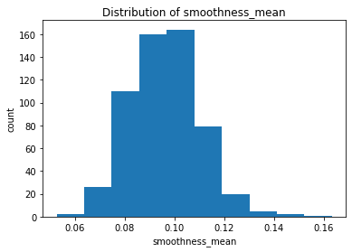
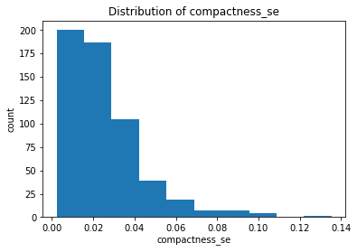
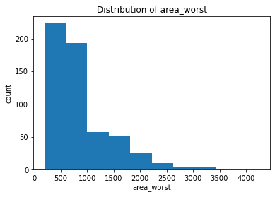
After plotting the distributions of all the features, we found that the majority of the mean features are roughly symmetric or normal whereas the majority of the se and worst features are relatively right-skewed.
Belign vs Malignant
Since we are interested in studying the difference between belign and malignant cancers, it might be helpful to analyze and compute the statistics of two populations separately and then compare.
belign = clean_data[clean_data['diagnosis'] == 0]
malignant = clean_data[clean_data['diagnosis'] == 1]
We first compare the means of each feature in two populations.
clean_data.groupby('diagnosis').mean().transpose()
| diagnosis | 0.0 | 1.0 |
|---|---|---|
| radius_mean | 12.146524 | 17.462830 |
| texture_mean | 17.914762 | 21.604906 |
| perimeter_mean | 78.075406 | 115.365377 |
| area_mean | 462.790196 | 978.376415 |
| smoothness_mean | 0.092478 | 0.102898 |
| compactness_mean | 0.080085 | 0.145188 |
| concavity_mean | 0.046058 | 0.160775 |
| concave points_mean | 0.025717 | 0.087990 |
| symmetry_mean | 0.174186 | 0.192909 |
| fractal_dimension_mean | 0.062867 | 0.062680 |
| radius_se | 0.284082 | 0.609083 |
| texture_se | 1.220380 | 1.210915 |
| perimeter_se | 2.000321 | 4.323929 |
| area_se | 21.135148 | 72.672406 |
| smoothness_se | 0.007196 | 0.006780 |
| compactness_se | 0.021438 | 0.032281 |
| concavity_se | 0.025997 | 0.041824 |
| concave points_se | 0.009858 | 0.015060 |
| symmetry_se | 0.020584 | 0.020472 |
| fractal_dimension_se | 0.003636 | 0.004062 |
| radius_worst | 13.379801 | 21.134811 |
| texture_worst | 23.515070 | 29.318208 |
| perimeter_worst | 87.005938 | 141.370330 |
| area_worst | 558.899440 | 1422.286321 |
| smoothness_worst | 0.124959 | 0.144845 |
| compactness_worst | 0.182673 | 0.374824 |
| concavity_worst | 0.166238 | 0.450606 |
| concave points_worst | 0.074444 | 0.182237 |
| symmetry_worst | 0.270246 | 0.323468 |
| fractal_dimension_worst | 0.079442 | 0.091530 |
Obviously, most of the features have different averages in two populations, but it is hard to tell whether such differences are significant or not. To assess this, we can compare the distributions of features in each population.
plt.figure()
plt.hist(belign['smoothness_mean'], alpha=0.5, label="belign")
plt.hist(malignant['smoothness_mean'], alpha=0.5, label="malignant")
plt.xlabel('smoothness_mean')
plt.ylabel('count')
plt.legend()
plt.title("Distributions of smoothness_mean in two populations")
plt.savefig("../figures/smoothness_mean_distr_two_popu")
plt.show()

plt.figure()
plt.hist(belign['compactness_se'], alpha=0.5, label="belign")
plt.hist(malignant['compactness_se'], alpha=0.5, label="malignant")
plt.xlabel('compactness_se')
plt.ylabel('count')
plt.legend()
plt.title("Distributions of compactness_se in two populations")
plt.savefig("../figures/compactness_se_distr_two_popu")
plt.show()

plt.figure()
plt.hist(belign['area_worst'], alpha=0.5, label="belign")
plt.hist(malignant['area_worst'], alpha=0.5, label="malignant")
plt.xlabel('area_worst')
plt.ylabel('count')
plt.title("Distributions of area_worse in two populations")
plt.savefig("../figures/area_worst_distr_two_popu")
plt.show()
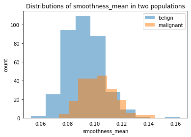
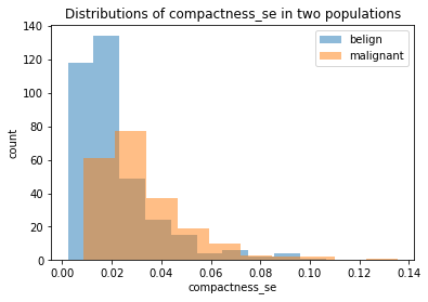
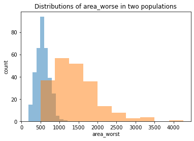
We chose the same three features we plotted before. We can see that although belign and malignant have different distributions in all the plots, it is still hard to judge whether it is due to the randomness since two populations have different size (as showed clearly in smoothness_mean feature). Thus, we should conduct some more rigorous statistical hypothesis testing, such as two-sample t-test, to judge this. And this will be done in a separate notebook called two-populations-analysis.ipynb.