Final Model Selection and Evaluation¶

In this notebook, we perform the model selection process between Logistic Regression model, Decision Tree model, and Random Forest model. Then, we evaluate the final model using the testing set and do the prediction analysis.

import numpy as np
import pandas as pd
import matplotlib.pyplot as plt
import seaborn as sns
import pickle
from sklearn.metrics import confusion_matrix, ConfusionMatrixDisplay, roc_curve, RocCurveDisplay, auc, precision_recall_curve, PrecisionRecallDisplay, f1_score
import matplotlib.image as mpimg
from IPython.display import Image

Load the Validation and Testing Data¶

val_data = pd.read_csv('../data/val.csv')
test_data = pd.read_csv('../data/test.csv')
X_val = val_data.drop(labels = ['diagnosis','id'],axis = 1)
y_val = val_data['diagnosis']
X_test = test_data.drop(labels = ['diagnosis','id'],axis = 1)
y_test = test_data['diagnosis']

Load Three Models from Disk¶

# load logistic model
model_lg = pickle.load(open('../models/lg_model.sav', 'rb'))
#  load random forest model
model_dt = pickle.load(open('../models/dt_model.sav', 'rb'))
# load random forest model
model_rf = pickle.load(open('../models/rf_model.sav', 'rb'))

Compare Metrics¶

We use validation data to obtain metrics that measure three models’ performance. We used the following metrics:

Accuracy: The accuray of a model is the fraction of correct predictions: \(\frac{\text{correct predictions}}{\text{total number of data points}}\)
Confusion Matrix: A confusion matrix is a table that is used to visualize the performance of a classification algorithm, with four elements: True Positive, True Negative, False Positve (Type I Error), False Negative (Type II Error)
ROC Curve: ROC curve is a graphical plot that illustrates the diagnostic ability of a binary classifier system as its discrimination threshold is varied. It shows the trade-off between sensitivity (or TPR) and specificity (1 – FPR).
Precision Recall Curve: The precision-recall curve is a graph with Precision values (\(\frac{TP}{TP+FN}\)) on the y-axis and Recall values (\(\frac{TP}{TP+FP}\)) on the x-axis. It shows the tradeoff between precision and recall for different threshold.
F1 score: F1 score combines the precision and recall of a classifier into a single metric by taking their harmonic mean. It is the weighted average of Precision and Recall. Therefore, this score takes both false positives and false negatives into account.

Accuracy¶

# accuracy of decision tree model and logistic regression model
rf_score = model_rf.score(X_val, y_val)
lg_score = model_lg.score(X_val, y_val)
dt_score = model_lg.score(X_val, y_val)
print("Decision Tree Model Accuracy: ", dt_score)
print("Random Forest Model Accuracy: ", rf_score)
print("Logistic Regression Accuracy: ", lg_score)

Decision Tree Model Accuracy:  0.9278350515463918
Random Forest Model Accuracy:  0.9587628865979382
Logistic Regression Accuracy:  0.9278350515463918

Random Forest Model does the best among three models in terms of accuracy.

Confusion Matrix¶

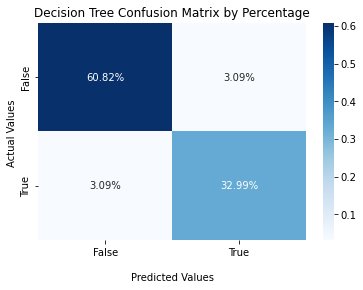
# Decision Tree Confusion Matrix
Image('../figures/confusion_matrix_dt.png')

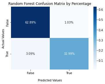
../_images/final_model_selection_12_0.png

# Random Forest Confusion Matrix
Image('../figures/confusion_matrix_rf.png')

../_images/final_model_selection_13_0.png

#Logistic Regression Confusion Matrix

cf_matrix_lg = confusion_matrix(y_val, model_lg.predict(X_val))

ax2 = sns.heatmap(cf_matrix_lg/np.sum(cf_matrix_lg), annot=True, 
            fmt='.2%', cmap='Blues')

ax2.set_title('Logistic Regression Confusion Matrix by Percentage');
ax2.set_xlabel('\nPredicted Values')
ax2.set_ylabel('Actual Values ');

ax2.xaxis.set_ticklabels(['False','True'])
ax2.yaxis.set_ticklabels(['False','True'])

plt.show();

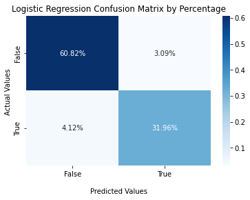
../_images/final_model_selection_14_0.png

From the above confusion matrices, Random Forest Model gets the highest TPR and TNR as well as the lowest FPR and FNR among three models.

ROC Curve¶

# Decision Tree ROC Curve
Image('../figures/roc_curve_dt.png')

../_images/final_model_selection_17_0.png

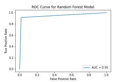
# Random Forest ROC Curve
Image('../figures/roc_curve_rf.png')

../_images/final_model_selection_18_0.png

# Logistic Regression ROC Curve
Image('../figures/roc_curve_logistic.png')

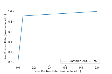
../_images/final_model_selection_19_0.png

Here we compare the AUC of two ROC curves. AUC stands for the area under an ROC curve, and it is a measure of the accuracy of a diagnostic test. AUC is the average true positive rate (average sensitivity) across all possible false positive rates. In general, higher AUC values indicate better test performance. In our case, Random Forest model has the highest AUC among three models.

Precision Recall Curve¶

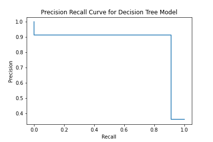
# Decision Tree Precision Recall Curve
Image('../figures/precision_recall_curve_dt.png')

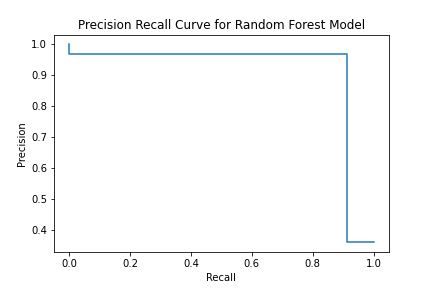
../_images/final_model_selection_22_0.png

# Random Forest Precision Recall Curve
Image('../figures/precision_recall_curve_rf.png')

../_images/final_model_selection_23_0.png

# Logistic Regression Precision Recall Curve
Image('../figures/precision_recall_curve_logistic.png')

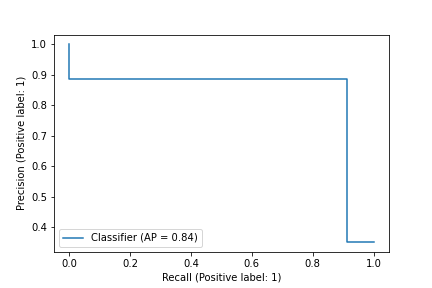
../_images/final_model_selection_24_0.png

We can observe that there is a larger area under Random Forest’s Precision Recall Curve than Logistic Regression’s curve and Decision Tree’s curve. Random Forest Model has both high recall and high precision.

F1 Score¶

f1_score_rf = f1_score(y_val, model_rf.predict(X_val))
f1_score_lg = f1_score(y_val, model_lg.predict(X_val))
f1_score_dt = f1_score(y_val, model_dt.predict(X_val))
print("Decision Tree F1 Score: ", f1_score_dt)
print("Random Forest Model F1 Score: ", f1_score_rf)
print("Logistic Regression F1 Score: ", f1_score_lg)

Decision Tree F1 Score:  0.9411764705882354
Random Forest Model F1 Score:  0.9411764705882354
Logistic Regression F1 Score:  0.8985507246376812

Random Forest Model has the highest F1 score.

# showing the summary table of metrics
d = {
    'Metrics': ['Accuracy', 'FPR', 'FNR', 'TPR', 'TNR', 'AUC', 'F1 Score'],
    'Logistic Regression': ['0.9278', '0.0309', '0.0412', '0.3196', '0.6082', '0.92', '0.8986'],
    'Decision Tree': ['0.9381', '0.0309', '0.0309', '0.3299', '0.6082', '0.95', '0.9143'],
    'Random Forest': ['0.9588', '0.0103', '0.0309', '0.3299', '0.6289', '0.95', '0.9412']
}
d = {
    'Model': ['Logistic Regression', 'Decision Tree', 'Random Forest'],
    'Accuracy': ['0.9278', '0.9381', '0.9588'],
    'FPR': ['0.0309', '0.0309', '0.0103'],
    'FNR': ['0.0412', '0.0309', '0.0309'],
    'TPR': ['0.3196', '0.3299', '0.3299'],
    'TNR': ['0.6082', '0.6082', '0.6289'],
    'AUC': ['0.92', '0.93', '0.95'],
    'F1 Score': ['0.8986', '0.9143', '0.9412']
}
metrics_df = pd.DataFrame(data=d)

# save the table to pickle file
metrics_df.to_pickle('../tables/metrics_df.pkl')

metrics_df

	Model	Accuracy	FPR	FNR	TPR	TNR	AUC	F1 Score
0	Logistic Regression	0.9278	0.0309	0.0412	0.3196	0.6082	0.92	0.8986
1	Decision Tree	0.9381	0.0309	0.0309	0.3299	0.6082	0.93	0.9143
2	Random Forest	0.9588	0.0103	0.0309	0.3299	0.6289	0.95	0.9412

By comparing metrices, Random Forest Model performs the best among three models in validation dataset. Therefore, we will select Random Forest Model as our final prediction model and use the test set to evaluate its performance.

Evaluation¶

y_pred_test = model_rf.predict(X_test)
# accuarcy
accuracy = model_rf.score(X_test, y_test)
print("The accuracy of our final model is: ", accuracy)

The accuracy of our final model is:  0.9534883720930233

# confusion matrix
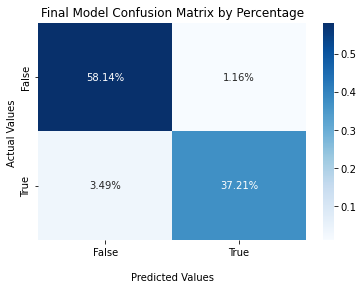
final_matrix = confusion_matrix(y_test, y_pred_test)

ax2 = sns.heatmap(final_matrix/np.sum(final_matrix), annot=True, 
            fmt='.2%', cmap='Blues')

ax2.set_title('Final Model Confusion Matrix by Percentage');
ax2.set_xlabel('\nPredicted Values')
ax2.set_ylabel('Actual Values ');

ax2.xaxis.set_ticklabels(['False','True'])
ax2.yaxis.set_ticklabels(['False','True'])

plt.savefig('../figures/confusion_matrix_final.png', bbox_inches = 'tight')
plt.show()

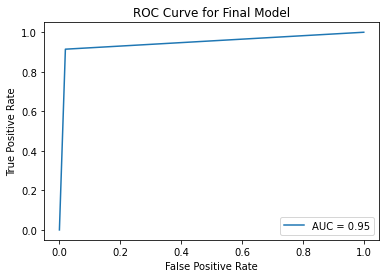
../_images/final_model_selection_33_0.png

# ROC curve
fpr, tpr, thresholds = roc_curve(y_test, y_pred_test)
roc_auc = auc(fpr, tpr)
display = RocCurveDisplay(fpr=fpr, tpr=tpr, roc_auc=roc_auc)
display.plot()
plt.title("ROC Curve for Final Model")

plt.savefig('../figures/roc_curve_final.png')
plt.show();

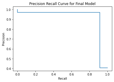
../_images/final_model_selection_34_0.png

# Precision Recall curve
precision, recall, _ = precision_recall_curve(y_test, y_pred_test)
disp = PrecisionRecallDisplay(precision=precision, recall=recall)
disp.plot()
plt.title("Precision Recall Curve for Final Model")

plt.savefig('../figures/precision_recall_curve_final.png')
plt.show();

../_images/final_model_selection_35_0.png

# F1 score
f1_score_final = f1_score(y_test, y_pred_test)
print("The F1 socre of our final model is: ", f1_score_final)

The F1 socre of our final model is:  0.9411764705882354

Overall, we are able to build a prediction model that has high accuracy and balances precision and recall. One notable thing of our model is that it has a relatively higher False Negative Rate than False Positive Rate, which means it is more likely to identifiy a patient who actually has malignant breast cancer as having benign breast cancer. In future studies, we might focus on how to lower the FNR when building the predictive model.

Breast Cancer Data Study

Final Model Selection and Evaluation

Contents