Two Populations Comparative Statistical Analysis
Two Populations Comparative Statistical Analysis
This notebook explores the differences between two populations: patients with malignant breast cancer and those with benign breast cancer. We have a sample of 357 patients with benign cancer and 212 patients with malignant cancer consisting of 30 key variables that may help distinguish key features between these two populations which may help to better identify cancer in patients. We will utilize hypothesis testing to see whether the two groups do indeed differ in some key features which is not due to chance.
import pandas as pd
import matplotlib.pyplot as plt
from diagnosis.twosample import plt_by_diagnosis, two_sample_t_test
dat = pd.read_csv('../data/clean.csv')
dat_ = dat.iloc[:, 1:]
dat.head()
| id | diagnosis | radius_mean | texture_mean | perimeter_mean | area_mean | smoothness_mean | compactness_mean | concavity_mean | concave points_mean | ... | radius_worst | texture_worst | perimeter_worst | area_worst | smoothness_worst | compactness_worst | concavity_worst | concave points_worst | symmetry_worst | fractal_dimension_worst | |
|---|---|---|---|---|---|---|---|---|---|---|---|---|---|---|---|---|---|---|---|---|---|
| 0 | 842302 | 1.0 | 17.99 | 10.38 | 122.80 | 1001.0 | 0.11840 | 0.27760 | 0.3001 | 0.14710 | ... | 25.38 | 17.33 | 184.60 | 2019.0 | 0.1622 | 0.6656 | 0.7119 | 0.2654 | 0.4601 | 0.11890 |
| 1 | 842517 | 1.0 | 20.57 | 17.77 | 132.90 | 1326.0 | 0.08474 | 0.07864 | 0.0869 | 0.07017 | ... | 24.99 | 23.41 | 158.80 | 1956.0 | 0.1238 | 0.1866 | 0.2416 | 0.1860 | 0.2750 | 0.08902 |
| 2 | 84300903 | 1.0 | 19.69 | 21.25 | 130.00 | 1203.0 | 0.10960 | 0.15990 | 0.1974 | 0.12790 | ... | 23.57 | 25.53 | 152.50 | 1709.0 | 0.1444 | 0.4245 | 0.4504 | 0.2430 | 0.3613 | 0.08758 |
| 3 | 84348301 | 1.0 | 11.42 | 20.38 | 77.58 | 386.1 | 0.14250 | 0.28390 | 0.2414 | 0.10520 | ... | 14.91 | 26.50 | 98.87 | 567.7 | 0.2098 | 0.8663 | 0.6869 | 0.2575 | 0.6638 | 0.17300 |
| 4 | 84358402 | 1.0 | 20.29 | 14.34 | 135.10 | 1297.0 | 0.10030 | 0.13280 | 0.1980 | 0.10430 | ... | 22.54 | 16.67 | 152.20 | 1575.0 | 0.1374 | 0.2050 | 0.4000 | 0.1625 | 0.2364 | 0.07678 |
5 rows × 32 columns
Below we see all of the features that are included in the data in regards to each patient. While we may conduct a hypothesis test for each of the features, instead we will choose a few so that we do not run into the issue of multiple testing which though may be corrected by using certain techniques. I specifically want to conduct a two sample t test on the feature that differs the most in the patients that are diagnosed vs. those that are not, and the feature that differs the least. We are using the average oberved value in the two samples as the measurement of difference in the two populations. Additionally, we have also computed the standard deviation for each feature in the two populations, as the two sample t test differs for whether the two populations are assumed to have the same variance or not.
There are two assumptions that must be met in order to properly conduct a two sample t test which are (1) independent observations and (2) the data must be sampled from a Gaussian distribution. The first condition is true as we have independent observations of patients which are not influenced by other observations’ conditions. We will see in a bit whether the second assumption is met or not. If it is not, then we will conduct both the parametric two sample t test and the non-parametric Wilcoxon rank sum test.
dat.columns
Index(['id', 'diagnosis', 'radius_mean', 'texture_mean', 'perimeter_mean',
       'area_mean', 'smoothness_mean', 'compactness_mean', 'concavity_mean',
       'concave points_mean', 'symmetry_mean', 'fractal_dimension_mean',
       'radius_se', 'texture_se', 'perimeter_se', 'area_se', 'smoothness_se',
       'compactness_se', 'concavity_se', 'concave points_se', 'symmetry_se',
       'fractal_dimension_se', 'radius_worst', 'texture_worst',
       'perimeter_worst', 'area_worst', 'smoothness_worst',
       'compactness_worst', 'concavity_worst', 'concave points_worst',
       'symmetry_worst', 'fractal_dimension_worst'],
      dtype='object')
dat__diagnosis_mean = dat_.groupby("diagnosis").mean()
dat__diagnosis_mean
| radius_mean | texture_mean | perimeter_mean | area_mean | smoothness_mean | compactness_mean | concavity_mean | concave points_mean | symmetry_mean | fractal_dimension_mean | ... | radius_worst | texture_worst | perimeter_worst | area_worst | smoothness_worst | compactness_worst | concavity_worst | concave points_worst | symmetry_worst | fractal_dimension_worst | |
|---|---|---|---|---|---|---|---|---|---|---|---|---|---|---|---|---|---|---|---|---|---|
| diagnosis | |||||||||||||||||||||
| 0.0 | 12.146524 | 17.914762 | 78.075406 | 462.790196 | 0.092478 | 0.080085 | 0.046058 | 0.025717 | 0.174186 | 0.062867 | ... | 13.379801 | 23.515070 | 87.005938 | 558.899440 | 0.124959 | 0.182673 | 0.166238 | 0.074444 | 0.270246 | 0.079442 |
| 1.0 | 17.462830 | 21.604906 | 115.365377 | 978.376415 | 0.102898 | 0.145188 | 0.160775 | 0.087990 | 0.192909 | 0.062680 | ... | 21.134811 | 29.318208 | 141.370330 | 1422.286321 | 0.144845 | 0.374824 | 0.450606 | 0.182237 | 0.323468 | 0.091530 |
2 rows × 30 columns
dat__diagnosis_std = dat_.groupby("diagnosis").std()
dat__diagnosis_std
| radius_mean | texture_mean | perimeter_mean | area_mean | smoothness_mean | compactness_mean | concavity_mean | concave points_mean | symmetry_mean | fractal_dimension_mean | ... | radius_worst | texture_worst | perimeter_worst | area_worst | smoothness_worst | compactness_worst | concavity_worst | concave points_worst | symmetry_worst | fractal_dimension_worst | |
|---|---|---|---|---|---|---|---|---|---|---|---|---|---|---|---|---|---|---|---|---|---|
| diagnosis | |||||||||||||||||||||
| 0.0 | 1.780512 | 3.995125 | 11.807438 | 134.287118 | 0.013446 | 0.033750 | 0.043442 | 0.015909 | 0.024807 | 0.006747 | ... | 1.981368 | 5.493955 | 13.527091 | 163.601424 | 0.020013 | 0.092180 | 0.140368 | 0.035797 | 0.041745 | 0.013804 |
| 1.0 | 3.203971 | 3.779470 | 21.854653 | 367.937978 | 0.012608 | 0.053987 | 0.075019 | 0.034374 | 0.027638 | 0.007573 | ... | 4.283569 | 5.434804 | 29.457055 | 597.967743 | 0.021870 | 0.170372 | 0.181507 | 0.046308 | 0.074685 | 0.021553 |
2 rows × 30 columns
In the below table, we see that the ‘area worst’, which is the average of the three highest values of area for each patient, feature has the minimum difference and the ‘texture_se’, which is the stanadrd error of the texture variable for each patient, has the maximum difference. More so, it appears that ‘area worst’ has a different variance in the population while ‘texture se’ has thee same population variance.
dat__diagnosis_mean.loc["diff"] = dat__diagnosis_mean.loc[0] - dat__diagnosis_mean.loc[1]
dat__diagnosis_mean
| radius_mean | texture_mean | perimeter_mean | area_mean | smoothness_mean | compactness_mean | concavity_mean | concave points_mean | symmetry_mean | fractal_dimension_mean | ... | radius_worst | texture_worst | perimeter_worst | area_worst | smoothness_worst | compactness_worst | concavity_worst | concave points_worst | symmetry_worst | fractal_dimension_worst | |
|---|---|---|---|---|---|---|---|---|---|---|---|---|---|---|---|---|---|---|---|---|---|
| diagnosis | |||||||||||||||||||||
| 0.0 | 12.146524 | 17.914762 | 78.075406 | 462.790196 | 0.092478 | 0.080085 | 0.046058 | 0.025717 | 0.174186 | 0.062867 | ... | 13.379801 | 23.515070 | 87.005938 | 558.899440 | 0.124959 | 0.182673 | 0.166238 | 0.074444 | 0.270246 | 0.079442 |
| 1.0 | 17.462830 | 21.604906 | 115.365377 | 978.376415 | 0.102898 | 0.145188 | 0.160775 | 0.087990 | 0.192909 | 0.062680 | ... | 21.134811 | 29.318208 | 141.370330 | 1422.286321 | 0.144845 | 0.374824 | 0.450606 | 0.182237 | 0.323468 | 0.091530 |
| diff | -5.316306 | -3.690144 | -37.289971 | -515.586219 | -0.010421 | -0.065103 | -0.114717 | -0.062273 | -0.018723 | 0.000187 | ... | -7.755010 | -5.803138 | -54.364392 | -863.386881 | -0.019886 | -0.192152 | -0.284368 | -0.107793 | -0.053222 | -0.012088 |
3 rows × 30 columns
min_diff, max_diff = dat__diagnosis_mean.loc["diff"].min(), dat__diagnosis_mean.loc["diff"].max()
dat__diagnosis_mean.columns[dat__diagnosis_mean.loc["diff"] == min_diff][0]
'area_worst'
dat__diagnosis_mean.columns[dat__diagnosis_mean.loc["diff"] == max_diff][0]
'texture_se'
dat__diagnosis_mean["area_worst"]
diagnosis
0.0      558.899440
1.0     1422.286321
diff    -863.386881
Name: area_worst, dtype: float64
dat__diagnosis_std["area_worst"]
diagnosis
0.0    163.601424
1.0    597.967743
Name: area_worst, dtype: float64
dat__diagnosis_mean["texture_se"]
diagnosis
0.0     1.220380
1.0     1.210915
diff    0.009465
Name: texture_se, dtype: float64
dat__diagnosis_std["texture_se"]
diagnosis
0.0    0.589180
1.0    0.483178
Name: texture_se, dtype: float64
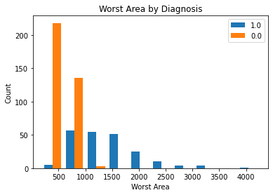
The below plot depicts the count distribution of ‘Worst Area’ for patients with malignant cancer and for those with benign cancer. We see that the patients with malignant cancer have a distribution with a higher variance, while those with benign cancer have a lower variance. We see that patients with benign cancer have a lower mean than those with malignant cancer. The distribution for the malignant cancer in blue below appears to be somewhat normally distrtibuted with a bit of a right tail; however, for th benign cancer patients, the worst area variable is concentrated to th left with a right tail. Overall, both distributions are not normally distributed. To combat this issue, we will perform both the parametric and the non-parametric hypothesis tests.
plt_by_diagnosis(dat, "area_worst", "Worst Area")
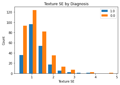
The below plot depicts the count distribution of ‘Texture SE for patients with malignant cancer and for those with benign cancer. We see that the patients with malignant cancer have a very similar to those with benign cancer We see that patients with benign cancer have a slighlty longer right tail than those with malignant cancer. Both distributions depictted below appear to be approximately normally distributed, though they do have a right-skewed tail. Though one may argue that the distributions below are approximately normally distributed and that the two sample t test will work, either way, we will perform both the parametric and the non-parametric hypothesis tests.
plt_by_diagnosis(dat, "texture_se", "Texture SE")
We are perforrming the below hypothesis tests with an alpha of 0.05.
We see that the two sample t test for ‘area worst’ is statistically highly significant at alpha = 0.05 with a p-value very close to zero. More so, the non-parametric Wilcoxian rank sum test agrees with the outcome of the parametric test. This means that we reject the null hypothesis that the two populations have a different area worst mean, which means that doctors may utilize this variable as an indicator of benign vs malignant cancer.
area_worst_ht_p = two_sample_t_test(dat, "diagnosis", "area_worst", False, True)
area_worst_ht_p
Statistically Highly Significant, Reject Null Hypohesis
Ttest_indResult(statistic=-20.570814251119344, pvalue=4.937923843586185e-54)
area_worst_ht_np = two_sample_t_test(dat, "diagnosis", "area_worst", False, False)
area_worst_ht_np
Statistically Highly Significant, Reject Null Hypohesis
RanksumsResult(statistic=-18.75402925190002, pvalue=1.7946452985715502e-78)
We see that the two sample t test for ‘texture se’ is not statistically significant at alpha = 0.05 with a p-value of approximately 0.84. More so, the non-parametric Wilcoxian rank sum test agrees with the outcome of the parametriic test. This means that we fail to reject the null hypothesis that the two populations have the same area worst mean, which means that doctors may not find utilizing this variable as an indicator of benign vs malignant cancer too helpful.
texture_se_ht_p = two_sample_t_test(dat, "diagnosis", "texture_se", True, True)
texture_se_ht_p
Fail to Reject Null Hypohesis
Ttest_indResult(statistic=0.1977238031013334, pvalue=0.8433320287670163)
texture_se_ht_np = two_sample_t_test(dat, "diagnosis", "texture_se", True, False)
texture_se_ht_np
Fail to Reject Null Hypohesis
RanksumsResult(statistic=-0.46280525524255145, pvalue=0.6435039640045692)
ht_dt = pd.DataFrame({"area worst parametric": area_worst_ht_p, "area worst non-parametric": area_worst_ht_np, "texture se parametric": texture_se_ht_p, "texture se non-parametric": texture_se_ht_np}).T
ht_dt.columns = ["T Statistic", "P Value"]
ht_dt.to_pickle("../tables/ht_results.pkl")