Predicting Concentrations of PM2.5
Contents
Predicting Concentrations of PM2.5
import openaq
import pandas as pd
import numpy as np
import matplotlib.pyplot as plt
from sklearn.preprocessing import RobustScaler
from aqtools import aqutils as u

from tensorflow.keras import Sequential
from tensorflow.keras.layers import Dense, GRU
from tensorflow.keras.callbacks import EarlyStopping, ModelCheckpoint
from tensorflow.keras.optimizers import SGD

from noaa_sdk import noaa

api = openaq.OpenAQ()
Version 1
# Parameter setting

date_from = '2021-09-01T00:00:00Z' # Default: PST
date_to = '2022-03-01T00:00:00Z'
city = 'San Francisco-Oakland-Fremont'
location = 'Oakland'
data_query_limit = 4000
"""
Important! You may get 'ApiError: A bad request was made: 500'.
It's not because of our code but  of API server issue.
Please take a moment, and retry executing the cell.
"""
# co
pollutant = 'co'
status, resp = api.measurements(city=city,
                                location=location, parameter=pollutant,
                                date_from=date_from,
                                date_to=date_to,
                                limit=data_query_limit)
r = resp['results']
df_co = u.date_pollutant_value(r, pollutant)
df_co.head(3)
| date | co | |
|---|---|---|
| 3600 | 2021-08-31 17:00:00 | 0.3 |
| 3599 | 2021-08-31 18:00:00 | 0.3 |
| 3598 | 2021-08-31 19:00:00 | 0.3 |
# no2
pollutant = 'no2'
status, resp = api.measurements(city=city,
                                location=location, parameter=pollutant,
                                date_from=date_from,
                                date_to=date_to,
                                limit=data_query_limit)
r = resp['results']
df_no2 = u.date_pollutant_value(r, pollutant)

df_no2.head(3)
| date | no2 | |
|---|---|---|
| 3599 | 2021-08-31 17:00:00 | 0.002 |
| 3598 | 2021-08-31 18:00:00 | 0.003 |
| 3597 | 2021-08-31 19:00:00 | 0.004 |
# o3
pollutant = 'o3'
status, resp = api.measurements(city=city,
                                location=location, parameter=pollutant,
                                date_from=date_from,
                                date_to=date_to,
                                limit=data_query_limit)
r = resp['results']
df_o3 = pd.DataFrame(data=r)
df_o3 = u.date_pollutant_value(r, pollutant)

df_o3.head(3)
| date | o3 | |
|---|---|---|
| 3600 | 2021-08-31 17:00:00 | 0.031 |
| 3599 | 2021-08-31 18:00:00 | 0.031 |
| 3598 | 2021-08-31 19:00:00 | 0.030 |
# pm25
pollutant = 'pm25'
status, resp = api.measurements(city=city,
                                location=location, parameter=pollutant,
                                date_from=date_from,
                                date_to=date_to,
                                limit=data_query_limit)
r = resp['results']
df_pm25 = pd.DataFrame(data=r)
df_pm25 = u.date_pollutant_value(r, pollutant)

df_pm25.head(3)
| date | pm25 | |
|---|---|---|
| 3751 | 2021-08-31 17:00:00 | 11 |
| 3750 | 2021-08-31 18:00:00 | 12 |
| 3749 | 2021-08-31 19:00:00 | 15 |
# Merge dataframes on 'date' (find the intersection of values based on 'date')
df = df_co.merge(df_no2, how='inner', on='date')
df = df.merge(df_o3, how='inner', on='date')
df = df.merge(df_pm25, how='inner', on='date')
df = df.set_index(['date'])
df
| co | no2 | o3 | pm25 | |
|---|---|---|---|---|
| date | ||||
| 2021-08-31 17:00:00 | 0.30 | 0.002 | 0.031 | 11 |
| 2021-08-31 18:00:00 | 0.30 | 0.003 | 0.031 | 12 |
| 2021-08-31 19:00:00 | 0.30 | 0.004 | 0.030 | 15 |
| 2021-08-31 20:00:00 | 0.36 | 0.006 | 0.029 | 14 |
| 2021-08-31 21:00:00 | 0.37 | 0.006 | 0.028 | 12 |
| ... | ... | ... | ... | ... |
| 2022-02-28 12:00:00 | 0.47 | 0.025 | 0.023 | 15 |
| 2022-02-28 13:00:00 | 0.46 | 0.025 | 0.026 | 20 |
| 2022-02-28 14:00:00 | 0.38 | 0.016 | 0.038 | 13 |
| 2022-02-28 15:00:00 | 0.32 | 0.012 | 0.043 | 9 |
| 2022-02-28 16:00:00 | 0.30 | 0.011 | 0.040 | 6 |
3526 rows × 4 columns
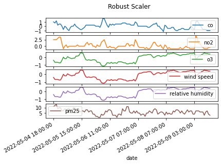
# MinMax Scaling
scaler = RobustScaler()
co_scaled = scaler.fit_transform(df['co'].values.reshape(-1, 1))
df['co'] = co_scaled

scaler = RobustScaler()
co_scaled = scaler.fit_transform(df['no2'].values.reshape(-1, 1))
df['no2'] = co_scaled

scaler = RobustScaler()
co_scaled = scaler.fit_transform(df['o3'].values.reshape(-1, 1))
df['o3'] = co_scaled

df.plot(subplots=True, title='Robust Scaler')
fig = plt.gcf()
fig.autofmt_xdate()
fig.savefig("./figures/scaling_ver1.png")
plt.show()
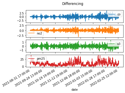
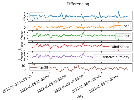
# Make data stationary
# Differencing technique was applied

co_diff = u.differencing(df['co'].values)
no2_diff = u.differencing(df['no2'].values)
o3_diff = u.differencing(df['o3'].values)
# Delete the first row
df = df.iloc[:-1, :]

df['co'] = co_diff
df['no2'] = no2_diff
df['o3'] = o3_diff
df.plot(subplots=True, title='Differencing')
fig = plt.gcf()
fig.autofmt_xdate()
fig.savefig("./figures/differencing_ver1.png")
plt.show()
/tmp/ipykernel_7700/3874090531.py:10: SettingWithCopyWarning:
A value is trying to be set on a copy of a slice from a DataFrame.
Try using .loc[row_indexer,col_indexer] = value instead

See the caveats in the documentation: https://pandas.pydata.org/pandas-docs/stable/user_guide/indexing.html#returning-a-view-versus-a-copy
  df['co'] = co_diff
/tmp/ipykernel_7700/3874090531.py:11: SettingWithCopyWarning:
A value is trying to be set on a copy of a slice from a DataFrame.
Try using .loc[row_indexer,col_indexer] = value instead

See the caveats in the documentation: https://pandas.pydata.org/pandas-docs/stable/user_guide/indexing.html#returning-a-view-versus-a-copy
  df['no2'] = no2_diff
/tmp/ipykernel_7700/3874090531.py:12: SettingWithCopyWarning:
A value is trying to be set on a copy of a slice from a DataFrame.
Try using .loc[row_indexer,col_indexer] = value instead

See the caveats in the documentation: https://pandas.pydata.org/pandas-docs/stable/user_guide/indexing.html#returning-a-view-versus-a-copy
  df['o3'] = o3_diff
# correlation among features
df_corr = df.corr()
df_corr.to_csv('./tables/correlation_ver1.csv')
df_corr
| co | no2 | o3 | pm25 | |
|---|---|---|---|---|
| co | 1.000000 | 0.673827 | -0.623135 | -0.118771 |
| no2 | 0.673827 | 1.000000 | -0.770821 | -0.113108 |
| o3 | -0.623135 | -0.770821 | 1.000000 | 0.080400 |
| pm25 | -0.118771 | -0.113108 | 0.080400 | 1.000000 |
# feature vectors: shape (num of data, window size, num of features)
feature_np = df[['co', 'no2', 'o3']].to_numpy()

# label vactors: shape (num of data,)
label_np = df[['pm25']].to_numpy()
X = []
y = []

# how many timesteps we want to look at --> default 8 (hours)
for i in range(8, len(feature_np)):
    X.append(feature_np[i-8:i, :])
    y.append(label_np[i])

X, y = np.array(X, dtype=np.float64), np.array(y, dtype=np.float64)
X.shape, y.shape
((3517, 8, 3), (3517, 1))
TEST_SIZE = 300

X_train = X[:-TEST_SIZE]
y_train = y[:-TEST_SIZE]
X_test = X[-TEST_SIZE:]
y_test = y[-TEST_SIZE:]


X_train.shape, y_train.shape, X_test.shape, y_test.shape
((3217, 8, 3), (3217, 1), (300, 8, 3), (300, 1))
# Predict pm2.5 using Gated Recurrent Unit

model = Sequential()
model.add(GRU(units=50,
              return_sequences=True,
              input_shape=X_train[0].shape,
              activation='tanh'))
model.add(GRU(units=50, activation='tanh'))
model.add(Dense(units=2))

# Compiling the GRU
model.compile(optimizer=SGD(learning_rate=0.01, decay=1e-7,
                            momentum=0.9, nesterov=False),
              loss='mse')

model.summary()
2022-05-12 03:39:34.489909: I tensorflow/core/platform/cpu_feature_guard.cc:151] This TensorFlow binary is optimized with oneAPI Deep Neural Network Library (oneDNN) to use the following CPU instructions in performance-critical operations:  SSE4.1 SSE4.2 AVX AVX2 FMA
To enable them in other operations, rebuild TensorFlow with the appropriate compiler flags.
Model: "sequential"
_________________________________________________________________
 Layer (type)                Output Shape              Param #
=================================================================
 gru (GRU)                   (None, 8, 50)             8250

 gru_1 (GRU)                 (None, 50)                15300

 dense (Dense)               (None, 2)                 102

=================================================================
Total params: 23,652
Trainable params: 23,652
Non-trainable params: 0
_________________________________________________________________
# model training
#early_stop = EarlyStopping(monitor='loss', mode='min', verbose=0, patience=10)
#model.fit(X_train, y_train, epochs=100, batch_size=150, verbose=1, callbacks=[early_stop])

model.fit(X_train, y_train, epochs=100, batch_size=150, verbose=1)
Epoch 1/100
22/22 [==============================] - 3s 15ms/step - loss: 61.7825
Epoch 2/100
22/22 [==============================] - 0s 14ms/step - loss: 47.2600
Epoch 3/100
22/22 [==============================] - 0s 15ms/step - loss: 46.5220
Epoch 4/100
22/22 [==============================] - 0s 14ms/step - loss: 46.0431
Epoch 5/100
22/22 [==============================] - 0s 14ms/step - loss: 45.9086
Epoch 6/100
22/22 [==============================] - 0s 14ms/step - loss: 45.9669
Epoch 7/100
22/22 [==============================] - 0s 14ms/step - loss: 46.2019
Epoch 8/100
22/22 [==============================] - 0s 13ms/step - loss: 43.4890
Epoch 9/100
22/22 [==============================] - 0s 14ms/step - loss: 41.3602
Epoch 10/100
22/22 [==============================] - 0s 15ms/step - loss: 39.4300
Epoch 11/100
22/22 [==============================] - 0s 15ms/step - loss: 38.2915
Epoch 12/100
22/22 [==============================] - 0s 15ms/step - loss: 40.1313
Epoch 13/100
22/22 [==============================] - 0s 15ms/step - loss: 37.6508
Epoch 14/100
22/22 [==============================] - 0s 14ms/step - loss: 36.5795
Epoch 15/100
22/22 [==============================] - 0s 14ms/step - loss: 36.3274
Epoch 16/100
22/22 [==============================] - 0s 14ms/step - loss: 35.6911
Epoch 17/100
22/22 [==============================] - 0s 14ms/step - loss: 35.0691
Epoch 18/100
22/22 [==============================] - 0s 14ms/step - loss: 35.2598
Epoch 19/100
22/22 [==============================] - 0s 14ms/step - loss: 36.0980
Epoch 20/100
22/22 [==============================] - 0s 15ms/step - loss: 34.3189
Epoch 21/100
22/22 [==============================] - 0s 15ms/step - loss: 33.0377
Epoch 22/100
22/22 [==============================] - 0s 14ms/step - loss: 32.3313
Epoch 23/100
22/22 [==============================] - 0s 14ms/step - loss: 31.3445
Epoch 24/100
22/22 [==============================] - 0s 14ms/step - loss: 30.9620
Epoch 25/100
22/22 [==============================] - 0s 15ms/step - loss: 29.8989
Epoch 26/100
22/22 [==============================] - 0s 16ms/step - loss: 28.9788
Epoch 27/100
22/22 [==============================] - 0s 14ms/step - loss: 28.2696
Epoch 28/100
22/22 [==============================] - 0s 14ms/step - loss: 27.7180
Epoch 29/100
22/22 [==============================] - 0s 14ms/step - loss: 28.8570
Epoch 30/100
22/22 [==============================] - 0s 15ms/step - loss: 26.2209
Epoch 31/100
22/22 [==============================] - 0s 15ms/step - loss: 25.1053
Epoch 32/100
22/22 [==============================] - 0s 15ms/step - loss: 24.3861
Epoch 33/100
22/22 [==============================] - 0s 14ms/step - loss: 23.9058
Epoch 34/100
22/22 [==============================] - 0s 15ms/step - loss: 23.0863
Epoch 35/100
22/22 [==============================] - 0s 14ms/step - loss: 22.9559
Epoch 36/100
22/22 [==============================] - 0s 14ms/step - loss: 22.4067
Epoch 37/100
22/22 [==============================] - 0s 15ms/step - loss: 19.7727
Epoch 38/100
22/22 [==============================] - 0s 15ms/step - loss: 18.2430
Epoch 39/100
22/22 [==============================] - 0s 14ms/step - loss: 16.6916
Epoch 40/100
22/22 [==============================] - 0s 15ms/step - loss: 17.0721
Epoch 41/100
22/22 [==============================] - 0s 14ms/step - loss: 17.3268
Epoch 42/100
22/22 [==============================] - 0s 15ms/step - loss: 16.3780
Epoch 43/100
22/22 [==============================] - 0s 14ms/step - loss: 14.5547
Epoch 44/100
22/22 [==============================] - 0s 15ms/step - loss: 13.6701
Epoch 45/100
22/22 [==============================] - 0s 15ms/step - loss: 13.8296
Epoch 46/100
22/22 [==============================] - 0s 14ms/step - loss: 13.4327
Epoch 47/100
22/22 [==============================] - 0s 15ms/step - loss: 12.2368
Epoch 48/100
22/22 [==============================] - 0s 15ms/step - loss: 11.6621
Epoch 49/100
22/22 [==============================] - 0s 14ms/step - loss: 10.4138
Epoch 50/100
22/22 [==============================] - 0s 15ms/step - loss: 9.2011
Epoch 51/100
22/22 [==============================] - 0s 15ms/step - loss: 9.1597
Epoch 52/100
22/22 [==============================] - 0s 15ms/step - loss: 8.2274
Epoch 53/100
22/22 [==============================] - 0s 16ms/step - loss: 7.9333
Epoch 54/100
22/22 [==============================] - 0s 15ms/step - loss: 7.3819
Epoch 55/100
22/22 [==============================] - 0s 15ms/step - loss: 7.3128
Epoch 56/100
22/22 [==============================] - 0s 15ms/step - loss: 6.6691
Epoch 57/100
22/22 [==============================] - 0s 15ms/step - loss: 6.8974
Epoch 58/100
22/22 [==============================] - 0s 15ms/step - loss: 6.2350
Epoch 59/100
22/22 [==============================] - 0s 15ms/step - loss: 5.3208
Epoch 60/100
22/22 [==============================] - 0s 15ms/step - loss: 5.3226
Epoch 61/100
22/22 [==============================] - 0s 15ms/step - loss: 4.9757
Epoch 62/100
22/22 [==============================] - 0s 15ms/step - loss: 4.7543
Epoch 63/100
22/22 [==============================] - 0s 16ms/step - loss: 4.3134
Epoch 64/100
22/22 [==============================] - 0s 15ms/step - loss: 3.9720
Epoch 65/100
22/22 [==============================] - 0s 15ms/step - loss: 3.4406
Epoch 66/100
22/22 [==============================] - 0s 16ms/step - loss: 3.1337
Epoch 67/100
22/22 [==============================] - 0s 15ms/step - loss: 3.2613
Epoch 68/100
22/22 [==============================] - 0s 15ms/step - loss: 4.1395
Epoch 69/100
22/22 [==============================] - 0s 15ms/step - loss: 4.7379
Epoch 70/100
22/22 [==============================] - 0s 14ms/step - loss: 4.3833
Epoch 71/100
22/22 [==============================] - 0s 15ms/step - loss: 3.7696
Epoch 72/100
22/22 [==============================] - 0s 15ms/step - loss: 3.3501
Epoch 73/100
22/22 [==============================] - 0s 16ms/step - loss: 2.7507
Epoch 74/100
22/22 [==============================] - 0s 15ms/step - loss: 2.3119
Epoch 75/100
22/22 [==============================] - 0s 15ms/step - loss: 1.9574
Epoch 76/100
22/22 [==============================] - 0s 14ms/step - loss: 1.7500
Epoch 77/100
22/22 [==============================] - 0s 14ms/step - loss: 1.7945
Epoch 78/100
22/22 [==============================] - 0s 15ms/step - loss: 1.7374
Epoch 79/100
22/22 [==============================] - 0s 14ms/step - loss: 1.5639
Epoch 80/100
22/22 [==============================] - 0s 15ms/step - loss: 1.4988
Epoch 81/100
22/22 [==============================] - 0s 15ms/step - loss: 1.5989
Epoch 82/100
22/22 [==============================] - 0s 14ms/step - loss: 1.3911
Epoch 83/100
22/22 [==============================] - 0s 15ms/step - loss: 1.2364
Epoch 84/100
22/22 [==============================] - 0s 15ms/step - loss: 1.1558
Epoch 85/100
22/22 [==============================] - 0s 14ms/step - loss: 1.1362
Epoch 86/100
22/22 [==============================] - 0s 15ms/step - loss: 1.0861
Epoch 87/100
22/22 [==============================] - 0s 15ms/step - loss: 0.9349
Epoch 88/100
22/22 [==============================] - 0s 14ms/step - loss: 0.8588
Epoch 89/100
22/22 [==============================] - 0s 15ms/step - loss: 0.7909
Epoch 90/100
22/22 [==============================] - 0s 15ms/step - loss: 0.7393
Epoch 91/100
22/22 [==============================] - 0s 14ms/step - loss: 0.8159
Epoch 92/100
22/22 [==============================] - 0s 14ms/step - loss: 0.7322
Epoch 93/100
22/22 [==============================] - 0s 14ms/step - loss: 0.7075
Epoch 94/100
22/22 [==============================] - 0s 14ms/step - loss: 0.6991
Epoch 95/100
22/22 [==============================] - 0s 15ms/step - loss: 0.6262
Epoch 96/100
22/22 [==============================] - 0s 15ms/step - loss: 0.6037
Epoch 97/100
22/22 [==============================] - 0s 15ms/step - loss: 0.7232
Epoch 98/100
22/22 [==============================] - 0s 15ms/step - loss: 0.7145
Epoch 99/100
22/22 [==============================] - 0s 14ms/step - loss: 0.5586
Epoch 100/100
22/22 [==============================] - 0s 14ms/step - loss: 0.5060
<keras.callbacks.History at 0x7f66744f5100>
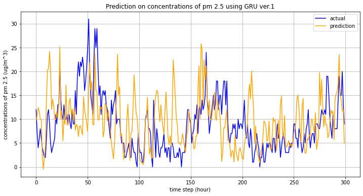
# Results for version 1
pred = model.predict(X_test)
pred = [p.mean() for p in pred]
plt.figure(figsize=(12, 6))
plt.plot(y_test, label='actual', color='blue')
plt.plot(pred, label='prediction', color='orange')
plt.title('Prediction on concentrations of pm 2.5 using GRU ver.1')
plt.xlabel('time step (hour)')
plt.ylabel('concentrations of pm 2.5 (ug/m^3)')
plt.grid()
plt.legend(loc='best')
plt.savefig('./figures/prediction_results_ver1.png')
plt.show()
Version 2
Regression with wind speed and relative humidity data
date_from = '2022-05-02T00:00:00Z'
date_to = '2022-05-10T00:00:00Z'
city = 'San Francisco-Oakland-Fremont'
location = 'Oakland'
data_query_limit = 150

date_from_utc = u.pst_to_utc(date_from)
date_to_utc = u.pst_to_utc(date_to)
# co
# From 2022-05-02 To 2022-05-10

pollutant = 'co'
status, resp = api.measurements(city=city,
                                location=location, parameter=pollutant,
                                date_from=date_from,
                                date_to=date_to,
                                limit=data_query_limit)
r = resp['results']
df_co = u.date_pollutant_value(r, pollutant)
df_co.head(3)
| date | co | |
|---|---|---|
| 149 | 2022-05-02 23:00:00 | 0.42 |
| 148 | 2022-05-03 00:00:00 | 0.29 |
| 147 | 2022-05-03 01:00:00 | 0.29 |
# no2
pollutant = 'no2'
status, resp = api.measurements(city=city,
                                location=location, parameter=pollutant,
                                date_from=date_from,
                                date_to=date_to,
                                limit=data_query_limit)
r = resp['results']
df_no2 = u.date_pollutant_value(r, pollutant)

df_no2.head(3)
| date | no2 | |
|---|---|---|
| 149 | 2022-05-02 23:00:00 | 0.013 |
| 148 | 2022-05-03 00:00:00 | 0.007 |
| 147 | 2022-05-03 01:00:00 | 0.006 |
# o3
pollutant = 'o3'
status, resp = api.measurements(city=city,
                                location=location, parameter=pollutant,
                                date_from=date_from,
                                date_to=date_to,
                                limit=data_query_limit)
r = resp['results']
df_o3 = pd.DataFrame(data=r)
df_o3 = u.date_pollutant_value(r, pollutant)

df_o3.head(3)
| date | o3 | |
|---|---|---|
| 149 | 2022-05-02 23:00:00 | 0.016 |
| 148 | 2022-05-03 00:00:00 | 0.019 |
| 147 | 2022-05-03 01:00:00 | 0.019 |
# pm25
pollutant = 'pm25'
status, resp = api.measurements(city=city,
                                location=location, parameter=pollutant,
                                date_from=date_from,
                                date_to=date_to,
                                limit=data_query_limit)
r = resp['results']
df_pm25 = pd.DataFrame(data=r)
df_pm25 = u.date_pollutant_value(r, pollutant)

df_pm25.head(3)
| date | pm25 | |
|---|---|---|
| 149 | 2022-05-03 04:00:00 | 8 |
| 148 | 2022-05-03 05:00:00 | 8 |
| 147 | 2022-05-03 06:00:00 | 7 |
# Collect NOAA (daily weather) data using NOAA Python SDK contributed by Paulo Kuong(2018)

n = noaa.NOAA()
res = n.get_observations('94603', 'US', start=date_from_utc, end=date_to_utc, num_of_stations=1)
dates = []
windspeed = []
relativehum = []

for i in res:
    dates.append(u.utc_to_pst(i['timestamp']))
    windspeed.append(i['windSpeed']['value'])
    relativehum.append(i['relativeHumidity']['value'])
df_w = pd.DataFrame()
df_w['date'] = dates
df_w['wind speed'] = windspeed
df_w['relative humidity'] = relativehum
df_w['date'] = pd.to_datetime(df_w['date'])

# fill na with median
df_w[['wind speed', 'relative humidity']] = df_w[['wind speed', 'relative humidity']].fillna(df_w[['wind speed', 'relative humidity']].median())
df_w = df_w.sort_values(by="date")
# df.to_csv('./fillna weather.csv')


df_w['date'] = df_w['date'].apply(lambda x: str(x).split('.', 1)[0].replace('T', ' '))

df_w.head(n=3)
| date | wind speed | relative humidity | |
|---|---|---|---|
| 72 | 2022-05-04 18:00:00 | 25.92 | 71.830366 |
| 52 | 2022-05-04 19:00:00 | 20.52 | 80.266011 |
| 43 | 2022-05-04 20:00:00 | 29.52 | 86.313549 |
# merge every dataframe on a date
df = df_co.merge(df_no2, how='inner', on='date')
df = df.merge(df_o3, how='inner', on='date')
df = df.merge(df_w,how='inner', on='date')
df = df.merge(df_pm25, how='inner', on='date')
df = df.set_index(['date'])
df
| co | no2 | o3 | wind speed | relative humidity | pm25 | |
|---|---|---|---|---|---|---|
| date | ||||||
| 2022-05-04 18:00:00 | 0.29 | 0.009 | 0.027 | 25.92 | 71.830366 | 11 |
| 2022-05-04 19:00:00 | 0.28 | 0.009 | 0.023 | 20.52 | 80.266011 | 12 |
| 2022-05-04 20:00:00 | 0.30 | 0.009 | 0.023 | 29.52 | 86.313549 | 13 |
| 2022-05-04 21:00:00 | 0.26 | 0.010 | 0.023 | 24.12 | 89.229634 | 9 |
| 2022-05-04 22:00:00 | 0.27 | 0.011 | 0.022 | 18.36 | 89.229634 | 10 |
| ... | ... | ... | ... | ... | ... | ... |
| 2022-05-09 12:00:00 | 0.22 | 0.002 | 0.041 | 25.92 | 47.248268 | 3 |
| 2022-05-09 13:00:00 | 0.22 | 0.002 | 0.040 | 18.36 | 43.875674 | 6 |
| 2022-05-09 14:00:00 | 0.21 | 0.002 | 0.040 | 27.72 | 43.875674 | 7 |
| 2022-05-09 15:00:00 | 0.21 | 0.003 | 0.039 | 25.92 | 42.044566 | 4 |
| 2022-05-09 16:00:00 | 0.21 | 0.003 | 0.039 | 18.36 | 45.606476 | 3 |
112 rows × 6 columns
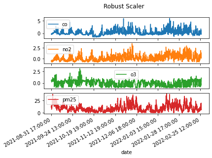
# Scaling
scaler = RobustScaler()
co_scaled = scaler.fit_transform(df['co'].values.reshape(-1, 1))
df['co'] = co_scaled

scaler = RobustScaler()
co_scaled = scaler.fit_transform(df['no2'].values.reshape(-1, 1))
df['no2'] = co_scaled

scaler = RobustScaler()
co_scaled = scaler.fit_transform(df['o3'].values.reshape(-1, 1))
df['o3'] = co_scaled

scaler = RobustScaler()
co_scaled = scaler.fit_transform(df['o3'].values.reshape(-1, 1))
df['wind speed'] = co_scaled

scaler = RobustScaler()
co_scaled = scaler.fit_transform(df['o3'].values.reshape(-1, 1))
df['relative humidity'] = co_scaled

plot = df.plot(subplots=True, title='Robust Scaler')
fig = plt.gcf()
fig.autofmt_xdate()
fig.savefig("./figures/scaling_ver2.png")
plt.show()
# Make data stationary
# Differencing technique was applied

co_diff = u.differencing(df['co'].values)
no2_diff = u.differencing(df['no2'].values)
o3_diff = u.differencing(df['o3'].values)
ws_diff = u.differencing(df['wind speed'].values)
rh_diff = u.differencing(df['relative humidity'].values)
# Delete the first row
df = df.iloc[:-1, :]

df['co'] = co_diff
df['no2'] = no2_diff
df['o3'] = o3_diff
df['wind speed'] = ws_diff
df['relative humidity'] = rh_diff
plot = df.plot(subplots=True, title='Differencing')
fig = plt.gcf()
fig.autofmt_xdate()
fig.savefig("./figures/differencing_ver2.png")
plt.show()
/tmp/ipykernel_7700/1728641024.py:12: SettingWithCopyWarning:
A value is trying to be set on a copy of a slice from a DataFrame.
Try using .loc[row_indexer,col_indexer] = value instead

See the caveats in the documentation: https://pandas.pydata.org/pandas-docs/stable/user_guide/indexing.html#returning-a-view-versus-a-copy
  df['co'] = co_diff
/tmp/ipykernel_7700/1728641024.py:13: SettingWithCopyWarning:
A value is trying to be set on a copy of a slice from a DataFrame.
Try using .loc[row_indexer,col_indexer] = value instead

See the caveats in the documentation: https://pandas.pydata.org/pandas-docs/stable/user_guide/indexing.html#returning-a-view-versus-a-copy
  df['no2'] = no2_diff
/tmp/ipykernel_7700/1728641024.py:14: SettingWithCopyWarning:
A value is trying to be set on a copy of a slice from a DataFrame.
Try using .loc[row_indexer,col_indexer] = value instead

See the caveats in the documentation: https://pandas.pydata.org/pandas-docs/stable/user_guide/indexing.html#returning-a-view-versus-a-copy
  df['o3'] = o3_diff
/tmp/ipykernel_7700/1728641024.py:15: SettingWithCopyWarning:
A value is trying to be set on a copy of a slice from a DataFrame.
Try using .loc[row_indexer,col_indexer] = value instead

See the caveats in the documentation: https://pandas.pydata.org/pandas-docs/stable/user_guide/indexing.html#returning-a-view-versus-a-copy
  df['wind speed'] = ws_diff
/tmp/ipykernel_7700/1728641024.py:16: SettingWithCopyWarning:
A value is trying to be set on a copy of a slice from a DataFrame.
Try using .loc[row_indexer,col_indexer] = value instead

See the caveats in the documentation: https://pandas.pydata.org/pandas-docs/stable/user_guide/indexing.html#returning-a-view-versus-a-copy
  df['relative humidity'] = rh_diff
# correlation among features
df_corr = df.corr()
df_corr.to_csv('./tables/correlation_ver2.csv')
df_corr
| co | no2 | o3 | wind speed | relative humidity | pm25 | |
|---|---|---|---|---|---|---|
| co | 1.000000 | 0.614983 | -0.587944 | -0.587944 | -0.587944 | -0.132807 |
| no2 | 0.614983 | 1.000000 | -0.796106 | -0.796106 | -0.796106 | -0.168784 |
| o3 | -0.587944 | -0.796106 | 1.000000 | 1.000000 | 1.000000 | 0.120429 |
| wind speed | -0.587944 | -0.796106 | 1.000000 | 1.000000 | 1.000000 | 0.120429 |
| relative humidity | -0.587944 | -0.796106 | 1.000000 | 1.000000 | 1.000000 | 0.120429 |
| pm25 | -0.132807 | -0.168784 | 0.120429 | 0.120429 | 0.120429 | 1.000000 |
# feature vectors: shape (num of data, window size, num of features)
feature_np = df[['co', 'no2', 'o3', 'wind speed', 'relative humidity']].to_numpy()

# label vactors: shape (num of data,)
label_np = df[['pm25']].to_numpy()
X = []
y = []

# how many timesteps we want to look at --> default 8 (hours)
for i in range(8, len(feature_np)):
    X.append(feature_np[i-8:i, :])
    y.append(label_np[i])

X, y = np.array(X, dtype=np.float64), np.array(y, dtype=np.float64)
X.shape, y.shape
((103, 8, 5), (103, 1))
TEST_SIZE = 30

X_train = X[:-TEST_SIZE]
y_train = y[:-TEST_SIZE]
X_test = X[-TEST_SIZE:]
y_test = y[-TEST_SIZE:]


X_train.shape, y_train.shape, X_test.shape, y_test.shape
((73, 8, 5), (73, 1), (30, 8, 5), (30, 1))
# Predict pm2.5 using Gated Recurrent Unit

model = Sequential()
model.add(GRU(units=50,
              return_sequences=True,
              input_shape=X_train[0].shape,
              activation='tanh'))
model.add(GRU(units=50, activation='tanh'))
model.add(Dense(units=2))

# Compiling the GRU
model.compile(optimizer=SGD(learning_rate=0.01, decay=1e-7,
                            momentum=0.9, nesterov=False),
              loss='mse')

model.summary()
Model: "sequential_1"
_________________________________________________________________
 Layer (type)                Output Shape              Param #
=================================================================
 gru_2 (GRU)                 (None, 8, 50)             8550

 gru_3 (GRU)                 (None, 50)                15300

 dense_1 (Dense)             (None, 2)                 102

=================================================================
Total params: 23,952
Trainable params: 23,952
Non-trainable params: 0
_________________________________________________________________
# model training
early_stop = EarlyStopping(monitor='loss', mode='min', verbose=0, patience=10)
model.fit(X_train, y_train, epochs=50, batch_size=100, verbose=1, callbacks=[early_stop])
Epoch 1/50
1/1 [==============================] - 3s 3s/step - loss: 39.2118
Epoch 2/50
1/1 [==============================] - 0s 16ms/step - loss: 35.9047
Epoch 3/50
1/1 [==============================] - 0s 15ms/step - loss: 30.0764
Epoch 4/50
1/1 [==============================] - 0s 15ms/step - loss: 22.2573
Epoch 5/50
1/1 [==============================] - 0s 15ms/step - loss: 13.3274
Epoch 6/50
1/1 [==============================] - 0s 15ms/step - loss: 6.6729
Epoch 7/50
1/1 [==============================] - 0s 14ms/step - loss: 6.5386
Epoch 8/50
1/1 [==============================] - 0s 15ms/step - loss: 10.8090
Epoch 9/50
1/1 [==============================] - 0s 16ms/step - loss: 12.7183
Epoch 10/50
1/1 [==============================] - 0s 15ms/step - loss: 10.1887
Epoch 11/50
1/1 [==============================] - 0s 15ms/step - loss: 6.9064
Epoch 12/50
1/1 [==============================] - 0s 15ms/step - loss: 5.9878
Epoch 13/50
1/1 [==============================] - 0s 14ms/step - loss: 7.1485
Epoch 14/50
1/1 [==============================] - 0s 13ms/step - loss: 8.6062
Epoch 15/50
1/1 [==============================] - 0s 13ms/step - loss: 8.9615
Epoch 16/50
1/1 [==============================] - 0s 13ms/step - loss: 7.9354
Epoch 17/50
1/1 [==============================] - 0s 13ms/step - loss: 6.3954
Epoch 18/50
1/1 [==============================] - 0s 13ms/step - loss: 5.6047
Epoch 19/50
1/1 [==============================] - 0s 13ms/step - loss: 6.0716
Epoch 20/50
1/1 [==============================] - 0s 13ms/step - loss: 7.0572
Epoch 21/50
1/1 [==============================] - 0s 13ms/step - loss: 7.4110
Epoch 22/50
1/1 [==============================] - 0s 14ms/step - loss: 6.8170
Epoch 23/50
1/1 [==============================] - 0s 13ms/step - loss: 5.9507
Epoch 24/50
1/1 [==============================] - 0s 14ms/step - loss: 5.5706
Epoch 25/50
1/1 [==============================] - 0s 14ms/step - loss: 5.7996
Epoch 26/50
1/1 [==============================] - 0s 14ms/step - loss: 6.2321
Epoch 27/50
1/1 [==============================] - 0s 12ms/step - loss: 6.4381
Epoch 28/50
1/1 [==============================] - 0s 13ms/step - loss: 6.2904
Epoch 29/50
1/1 [==============================] - 0s 14ms/step - loss: 5.9492
Epoch 30/50
1/1 [==============================] - 0s 13ms/step - loss: 5.6633
Epoch 31/50
1/1 [==============================] - 0s 14ms/step - loss: 5.5910
Epoch 32/50
1/1 [==============================] - 0s 14ms/step - loss: 5.7226
Epoch 33/50
1/1 [==============================] - 0s 13ms/step - loss: 5.9103
Epoch 34/50
1/1 [==============================] - 0s 13ms/step - loss: 5.9842
<keras.callbacks.History at 0x7f66806cc400>
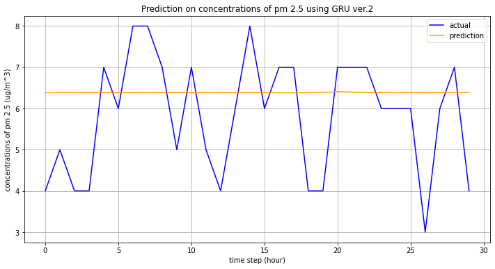
# Results for version 2
pred = model.predict(X_test)
pred = [p.mean() for p in pred]
plt.figure(figsize=(12, 6))
plt.plot(y_test, label='actual', color='blue')
plt.plot(pred, label='prediction', color='orange')
plt.title('Prediction on concentrations of pm 2.5 using GRU ver.2')
plt.xlabel('time step (hour)')
plt.ylabel('concentrations of pm 2.5 (ug/m^3)')
plt.grid()
plt.legend(loc='best')
plt.savefig('./figures/prediction_results_ver2.png')
plt.show()