Exploring and Visualizing OpenAQ Data
Contents
Exploring and Visualizing OpenAQ Data
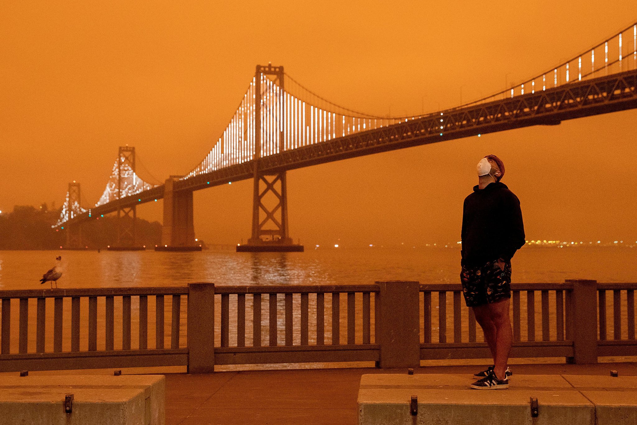
This notebook outlines the process that was taken for exploring the OpenAQ API and visualizing its data to learn more about air quality in the San Francisco Bay Area
import warnings
warnings.simplefilter(action='ignore', category=FutureWarning)
import openaq
import pandas as pd
import matplotlib.pyplot as plt
import seaborn as sns
import matplotlib as mpl
sns.set_theme(style="darkgrid")

import numpy as np
from shapely.geometry import Point

import geopandas as gpd
from geopandas import GeoDataFrame

import geoplot as gplt
import geoplot.crs as gcrs

import fiona

import imageio
import os

import IPython
from IPython.core.display import Image

from aqtools import viz_utils as vu
ERROR 1: PROJ: proj_create_from_database: Open of /home/jovyan/envs/aqproject/share/proj failed
There are several GIFs that are created from visualizations of the Bay Area over time. Due to memory constraints with the DataHub, the kernel crashes when animations are made, hence why the option is set to false by default. It can be set to true if one wishes to rebuild the animations (perhaps if you’re running a high performance computer)
# Set this to True if you want to create the animated figures; it can crash the kernel from creating too many plots however
animate = False
Exploring the OpenAQ API
api = openaq.OpenAQ()
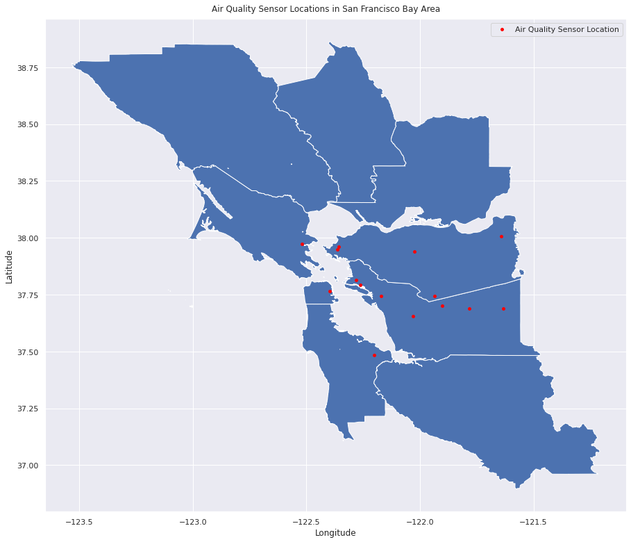
When we enter the OpenAQ API, we can filter the thousands of locations by the area we are interested in, the San Francisco Bay Area.
sanfrancisco = api.locations(city='San Francisco-Oakland-Fremont', df=True)
sanfrancisco
| id | country | city | cities | location | locations | sourceName | sourceNames | sourceType | sourceTypes | firstUpdated | lastUpdated | parameters | countsByMeasurement | count | coordinates.latitude | coordinates.longitude | |
|---|---|---|---|---|---|---|---|---|---|---|---|---|---|---|---|---|---|
| 0 | 1311 | US | San Francisco-Oakland-Fremont | [San Francisco-Oakland-Fremont] | Laney College | [Laney College] | AirNow | [AirNow] | government | [government] | 2016-03-06 19:00:00+00:00 | 2022-05-11 01:00:00+00:00 | [bc, no2, pm25, co] | [{'parameter': 'bc', 'count': 98488}, {'parame... | 382465 | 37.793624 | -122.263376 |
| 1 | 1518 | US | San Francisco-Oakland-Fremont | [San Francisco-Oakland-Fremont] | Livermore - Rincon | [Livermore - Rincon] | AirNow | [AirNow] | government | [government] | 2016-03-06 19:00:00+00:00 | 2022-05-11 01:00:00+00:00 | [pm25, o3, bc, no2] | [{'parameter': 'pm25', 'count': 97215}, {'para... | 373119 | 37.687526 | -121.784217 |
| 2 | 1520 | US | San Francisco-Oakland-Fremont | [San Francisco-Oakland-Fremont] | Bethel Island | [Bethel Island] | AirNow | [AirNow] | government | [government] | 2016-03-06 19:00:00+00:00 | 2022-05-11 01:00:00+00:00 | [no2, so2, o3, co] | [{'parameter': 'no2', 'count': 87339}, {'param... | 349902 | 38.006311 | -121.641918 |
| 3 | 1950 | US | San Francisco-Oakland-Fremont | [San Francisco-Oakland-Fremont] | Concord | [Concord] | AirNow | [AirNow] | government | [government] | 2016-03-06 19:00:00+00:00 | 2022-05-11 01:00:00+00:00 | [pm25, no2, co, o3, so2] | [{'parameter': 'pm25', 'count': 95358}, {'para... | 458098 | 37.938300 | -122.025000 |
| 4 | 2001 | US | San Francisco-Oakland-Fremont | [San Francisco-Oakland-Fremont] | San Ramon | [San Ramon] | AirNow | [AirNow] | government | [government] | 2016-04-01 17:00:00+00:00 | 2022-05-11 01:00:00+00:00 | [o3, no2] | [{'parameter': 'o3', 'count': 93595}, {'parame... | 186989 | 37.743649 | -121.934188 |
| 5 | 2002 | US | San Francisco-Oakland-Fremont | [San Francisco-Oakland-Fremont] | San Rafael | [San Rafael] | AirNow | [AirNow] | government | [government] | 2016-03-06 19:00:00+00:00 | 2022-05-11 01:00:00+00:00 | [o3, co, pm25, no2] | [{'parameter': 'o3', 'count': 92723}, {'parame... | 372510 | 37.972200 | -122.518900 |
| 6 | 2003 | US | San Francisco-Oakland-Fremont | [San Francisco-Oakland-Fremont] | San Pablo - Rumrill | [San Pablo - Rumrill] | AirNow | [AirNow] | government | [government] | 2016-03-06 19:00:00+00:00 | 2022-05-11 01:00:00+00:00 | [pm25, co, so2, o3, no2] | [{'parameter': 'pm25', 'count': 93676}, {'para... | 452238 | 37.960400 | -122.357100 |
| 7 | 2009 | US | San Francisco-Oakland-Fremont | [San Francisco-Oakland-Fremont] | San Francisco | [San Francisco] | AirNow | [AirNow] | government | [government] | 2016-03-06 19:00:00+00:00 | 2022-05-11 01:00:00+00:00 | [co, no2, pm25, o3] | [{'parameter': 'co', 'count': 91951}, {'parame... | 371070 | 37.765800 | -122.397800 |
| 8 | 2134 | US | San Francisco-Oakland-Fremont | [San Francisco-Oakland-Fremont] | Oakland | [Oakland] | AirNow | [AirNow] | government | [government] | 2016-03-06 19:00:00+00:00 | 2022-05-11 01:00:00+00:00 | [o3, no2, co, pm25] | [{'parameter': 'o3', 'count': 93203}, {'parame... | 375223 | 37.743061 | -122.169907 |
| 9 | 2135 | US | San Francisco-Oakland-Fremont | [San Francisco-Oakland-Fremont] | Oakland West | [Oakland West] | AirNow | [AirNow] | government | [government] | 2016-03-06 19:00:00+00:00 | 2022-05-11 01:00:00+00:00 | [o3, co, so2, pm25, bc, no2] | [{'parameter': 'o3', 'count': 90253}, {'parame... | 539170 | 37.814800 | -122.282402 |
| 10 | 2152 | US | San Francisco-Oakland-Fremont | [San Francisco-Oakland-Fremont] | Redwood City | [Redwood City] | AirNow | [AirNow] | government | [government] | 2016-03-06 19:00:00+00:00 | 2022-05-11 01:00:00+00:00 | [no2, co, o3, pm25] | [{'parameter': 'no2', 'count': 90807}, {'param... | 372762 | 37.482800 | -122.202200 |
| 11 | 8741 | US | San Francisco-Oakland-Fremont | [San Francisco-Oakland-Fremont] | Pleasanton - Owens C | [Pleasanton - Owens C] | AirNow | [AirNow] | government | [government] | 2018-05-14 20:00:00+00:00 | 2022-05-11 01:00:00+00:00 | [pm25, co, no2] | [{'parameter': 'pm25', 'count': 79253}, {'para... | 234229 | 37.701222 | -121.903019 |
| 12 | 8769 | US | San Francisco-Oakland-Fremont | [San Francisco-Oakland-Fremont] | Richmond - 7th St | [Richmond - 7th St] | AirNow | [AirNow] | government | [government] | 2016-07-26 13:00:00+00:00 | 2022-05-11 01:00:00+00:00 | [so2] | [{'parameter': 'so2', 'count': 86965}] | 86965 | 37.947800 | -122.363600 |
| 13 | 2035 | US | San Francisco-Oakland-Fremont | [San Francisco-Oakland-Fremont] | Hayward | [Hayward] | AirNow | [AirNow] | government | [government] | 2016-04-01 16:00:00+00:00 | 2022-05-10 23:00:00+00:00 | [o3] | [{'parameter': 'o3', 'count': 91964}] | 91964 | 37.654700 | -122.031700 |
| 14 | 1021 | US | San Francisco-Oakland-Fremont | [San Francisco-Oakland-Fremont] | Patterson Pass | [Patterson Pass] | AirNow | [AirNow] | government | [government] | 2016-03-06 19:00:00+00:00 | 2017-03-30 17:00:00+00:00 | [o3, no2] | [{'parameter': 'o3', 'count': 7054}, {'paramet... | 13902 | 37.689615 | -121.631916 |
geometry = [Point(xy) for xy in zip(sanfrancisco['coordinates.longitude'], sanfrancisco['coordinates.latitude'])]
gdf = GeoDataFrame(sanfrancisco, geometry=geometry)
world = gpd.read_file("https://data.sfgov.org/api/geospatial/s9wg-vcph?method=export&format=Shapefile")
gdf.plot(ax=world.plot(figsize=(15, 15)), marker='o', color='red', markersize=15, label="Air Quality Sensor Location")
plt.legend()
plt.xlabel("Longitude")
plt.ylabel("Latitude")
plt.suptitle("Air Quality Sensor Locations in San Francisco Bay Area", y=0.85)
plt.savefig('figures/BAgeog.png', dpi=300)
Now we can see what parameters are included with each packet of JSON data that comes from each location. Here is the set of parameters that comes from the San Francisco Air Quality Station.
param_file = sanfrancisco.iloc[7].to_frame().rename(columns={7:'San Francisco AQ Parameters'})
param_file.to_pickle('data/paramdf.pkl')
param_file
| San Francisco AQ Parameters | |
|---|---|
| id | 2009 |
| country | US |
| city | San Francisco-Oakland-Fremont |
| cities | [San Francisco-Oakland-Fremont] |
| location | San Francisco |
| locations | [San Francisco] |
| sourceName | AirNow |
| sourceNames | [AirNow] |
| sourceType | government |
| sourceTypes | [government] |
| firstUpdated | 2016-03-06 19:00:00+00:00 |
| lastUpdated | 2022-05-11 01:00:00+00:00 |
| parameters | [co, no2, pm25, o3] |
| countsByMeasurement | [{'parameter': 'co', 'count': 91951}, {'parame... |
| count | 371070 |
| coordinates.latitude | 37.7658 |
| coordinates.longitude | -122.3978 |
| geometry | POINT (-122.3978 37.7658) |
Now we’ll pull some summary statistics for the past week to see what the air quality has been like recently.
measure = api.measurements(city='San Francisco-Oakland-Fremont', date_from='2022-05-03',  date_to='2022-05-10', limit=10000, df=True)
# Print out the statistics on a per-location basis
def percentile(n):
    def percentile_(x):
        return np.percentile(x, n)
    percentile_.__name__ = '%sth percentile' % n
    return percentile_
stats = measure.groupby(['parameter'])['value'].agg(["min",  percentile(25),"median", "mean",percentile(75), "max"])
stats.to_pickle('data/weekstatsdf.pkl')
stats
| min | 25th percentile | median | mean | 75th percentile | max | |
|---|---|---|---|---|---|---|
| parameter | ||||||
| bc | 0.020 | 0.090 | 0.200 | 0.244613 | 0.315 | 1.170 |
| co | 0.120 | 0.220 | 0.280 | 0.312877 | 0.370 | 0.790 |
| no2 | 0.000 | 0.002 | 0.004 | 0.005016 | 0.006 | 0.036 |
| o3 | 0.003 | 0.025 | 0.034 | 0.032220 | 0.039 | 0.063 |
| pm25 | -3.000 | 4.000 | 6.000 | 6.339687 | 8.000 | 43.000 |
| so2 | -0.001 | 0.000 | 0.000 | 0.000491 | 0.001 | 0.012 |
Comparing current day to wildfire period
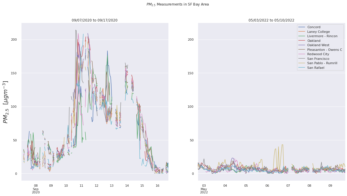
Now we’ll compare the current air quality to that during the wildfire period that caused the dark day, from 09/07/2020 to 09/17/2020.
pm25measure = api.measurements(city='San Francisco-Oakland-Fremont', param="pm25", date_from='2022-05-03', date_to='2022-05-10', limit=10000, df=True)
pm25measure = pm25measure[pm25measure['parameter'] == 'pm25']
dark_days_BA = api.measurements(city='San Francisco-Oakland-Fremont', param="pm25", date_from='2020-09-07', date_to='2020-09-17', limit=10000, df=True)
dark_days_BA = dark_days_BA[dark_days_BA['parameter'] == 'pm25']
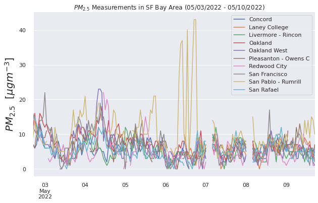
Plotting them on a time series and them comparing them, we can see that even the worst air quality (PM2.5 measurement specifically) days in the past week are not even a quarter of the worst air quality during the wildfire period.
fig, ax = plt.subplots(1, figsize=(10, 6))

for group, df in pm25measure.groupby('location'):
    # Query the data to only get positive values and resample to hourly
    _df = df.query("value >= 0.0").resample('1h').mean()
    _df.value.plot(ax=ax, label=group)

ax.legend(loc='best')
ax.set_ylabel("$PM_{2.5}$  [$\mu g m^{-3}$]", fontsize=20)
ax.set_xlabel("")
sns.despine(offset=5)


plt.suptitle("$PM_{2.5}$ Measurements in SF Bay Area (05/03/2022 - 05/10/2022)", y=0.92)

plt.savefig('figures/PM25TSthisweek.png', dpi=300)
plt.show()
fig= plt.figure(figsize=(20, 10))
ax1 = plt.subplot(121)
ax2 = plt.subplot(122, sharey=ax1)
for group, df in pm25measure.groupby('location'):
    # Query the data to only get positive values and resample to hourly
    _df = df.query("value >= 0.0").resample('1h').mean()
    _df.value.plot(ax=ax2, label=group)
for group, df in dark_days_BA.groupby('location'):
    # Query the data to only get positive values and resample to hourly
    _df = df.query("value >= 0.0").resample('1h').mean()
    _df.value.plot(ax=ax1, label=group)

plt.legend(loc='best')
ax1.set_ylabel("$PM_{2.5}$  [$\mu g m^{-3}$]", fontsize=20)
ax2.set_ylabel("$PM_{2.5}$  [$\mu g m^{-3}$]", fontsize=20)
ax1.set_xlabel("")
ax2.set_xlabel("")
sns.despine(offset=5)
ax1.set_title('09/07/2020 to 09/17/2020')
ax2.set_title('05/03/2022 to 05/10/2022')

plt.suptitle("$PM_{2.5}$ Measurements in SF Bay Area", y=0.98)
plt.savefig('figures/PM25TScompare.png', dpi=300)
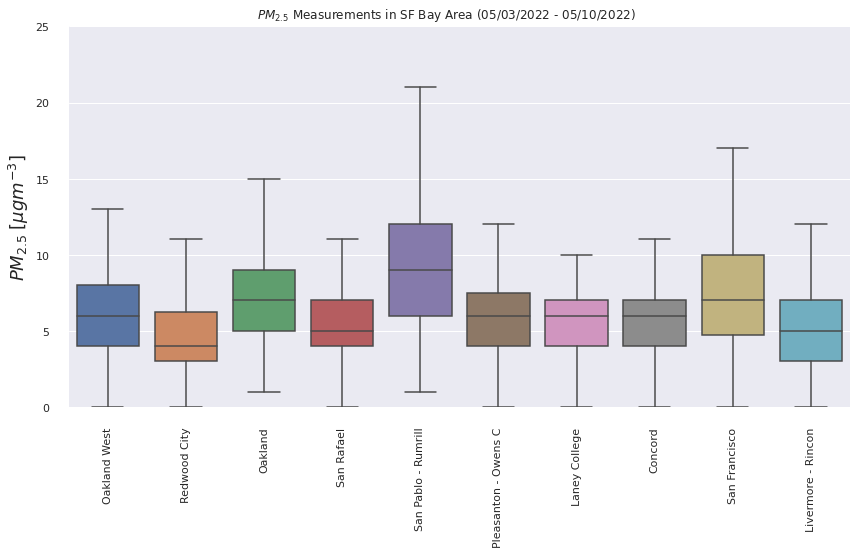
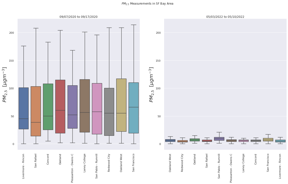
Comparing the summary statistics on a boxplot, we see similar results. The mean PM2.5 for the wildfire period across the Bay Area is about 10 times larger than that for the past week. This is good, as it means the poor air quality of that wildfire period was anomalous.
fig, ax = plt.subplots(1, figsize=(14,7))

ax = sns.boxplot(
    x='location',
    y='value',
    data=pm25measure.query("value >= 0.0"),
    fliersize=0,
    palette='deep',
    ax=ax)

ax.set_ylim([0, 25])
ax.set_ylabel("$PM_{2.5}\;[\mu gm^{-3}]$", fontsize=18)
ax.set_xlabel("")

sns.despine(offset=10)

plt.xticks(rotation=90)
plt.suptitle("$PM_{2.5}$ Measurements in SF Bay Area (05/03/2022 - 05/10/2022)", y=0.92)
plt.savefig('figures/PM25Boxthisweek.png', dpi=300)
fig= plt.figure(figsize=(20, 10))
ax1 = plt.subplot(121)
ax2 = plt.subplot(122, sharey=ax1)

ax2 = sns.boxplot(
    x='location',
    y='value',
    data=pm25measure.query("value >= 0.0"),
    fliersize=0,
    palette='deep',
    ax=ax2)

ax1 = sns.boxplot(
    x='location',
    y='value',
    data=dark_days_BA.query("value >= 0.0"),
    fliersize=0,
    palette='deep',
    ax=ax1)
plt.setp(ax1.get_xticklabels(), rotation=45)

ax1.tick_params(axis='x', labelrotation=90)
ax2.tick_params(axis='x', labelrotation=90)
ax1.set_ylabel("$PM_{2.5}$  [$\mu g m^{-3}$]", fontsize=20)
ax2.set_ylabel("$PM_{2.5}$  [$\mu g m^{-3}$]", fontsize=20)
ax1.set_xlabel("")
ax2.set_xlabel("")
sns.despine(offset=5)
ax1.set_title('09/07/2020 to 09/17/2020')
ax2.set_title('05/03/2022 to 05/10/2022')

plt.suptitle("$PM_{2.5}$ Measurements in SF Bay Area", y=0.98)
plt.savefig('figures/PM25Boxcompare.png', dpi=300)
Visualizing the wildfire period
dark_day_sf_pm25 = api.measurements(location='San Francisco', parameter='pm25', date_from='2020-09-07', date_to='2020-09-17', df=True, limit=1000)
dark_day_sf_pm25.head()
| location | parameter | value | unit | country | city | date.utc | coordinates.latitude | coordinates.longitude | |
|---|---|---|---|---|---|---|---|---|---|
| date.local | |||||||||
| 2020-09-16 17:00:00 | San Francisco | pm25 | -2 | b'\xc2\xb5g/m\xc2\xb3' | US | San Francisco-Oakland-Fremont | 2020-09-17 00:00:00+00:00 | 37.7658 | -122.3978 |
| 2020-09-16 16:00:00 | San Francisco | pm25 | -1 | b'\xc2\xb5g/m\xc2\xb3' | US | San Francisco-Oakland-Fremont | 2020-09-16 23:00:00+00:00 | 37.7658 | -122.3978 |
| 2020-09-16 15:00:00 | San Francisco | pm25 | 1 | b'\xc2\xb5g/m\xc2\xb3' | US | San Francisco-Oakland-Fremont | 2020-09-16 22:00:00+00:00 | 37.7658 | -122.3978 |
| 2020-09-16 14:00:00 | San Francisco | pm25 | 0 | b'\xc2\xb5g/m\xc2\xb3' | US | San Francisco-Oakland-Fremont | 2020-09-16 21:00:00+00:00 | 37.7658 | -122.3978 |
| 2020-09-16 09:00:00 | San Francisco | pm25 | 7 | b'\xc2\xb5g/m\xc2\xb3' | US | San Francisco-Oakland-Fremont | 2020-09-16 16:00:00+00:00 | 37.7658 | -122.3978 |
g = sns.relplot(x=dark_day_sf_pm25.index, y='value', kind='line', data=dark_day_sf_pm25, height=8.27, aspect=11.7/8.27)
g.fig.autofmt_xdate()
(g.map(plt.axhline, y=0, color=".7", dashes=(2, 1), zorder=0)
  .set_axis_labels("Date", "$PM_{2.5}\;[\mu gm^{-3}]$")
  .tight_layout(w_pad=0))

g.fig.suptitle('SF Particulate Matter 2.5 from Sept 7th to Sept 17th 2020', fontsize=20)
plt.savefig('figures/SFTS.png')
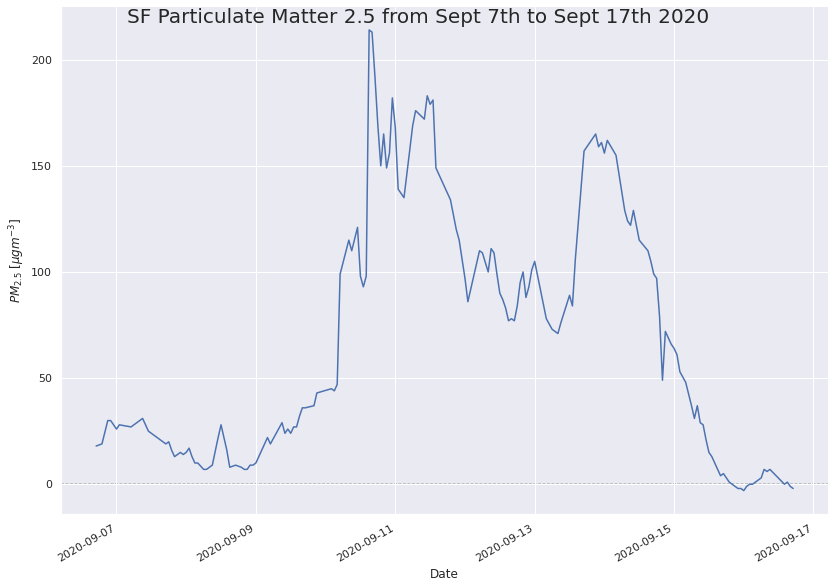
We see in the figure below that the PM2.5 levels during the wildfire period were bimodal in San Francisco, meaning the particulates likely moved and then returned via wind patterns. Let’s see if we can visualize where the particulates traveled to.
USlocs = api.locations(country='US', df=True, limit=10000)

USlocs.head()
| id | country | city | cities | location | locations | sourceName | sourceNames | sourceType | sourceTypes | firstUpdated | lastUpdated | parameters | countsByMeasurement | count | coordinates.latitude | coordinates.longitude | |
|---|---|---|---|---|---|---|---|---|---|---|---|---|---|---|---|---|---|
| 0 | 234 | US | WALLOWA | [WALLOWA] | Enterprise - US Fore | [Enterprise - US Fore] | AirNow | [AirNow] | government | [government] | 2016-03-10 08:00:00+00:00 | 2022-05-11 01:00:00+00:00 | [pm25] | [{'parameter': 'pm25', 'count': 80854}] | 80854 | 45.426351 | -117.296066 |
| 1 | 244 | US | Kansas City | [Kansas City] | LIBERTY | [LIBERTY] | AirNow | [AirNow] | government | [government] | 2016-03-06 19:00:00+00:00 | 2022-05-11 01:00:00+00:00 | [o3, pm25] | [{'parameter': 'o3', 'count': 64713}, {'parame... | 160119 | 39.303056 | -94.376389 |
| 2 | 255 | US | MONROE | [MONROE] | MTSP | [MTSP] | AirNow | [AirNow] | government | [government] | 2016-03-06 19:00:00+00:00 | 2022-05-11 01:00:00+00:00 | [pm10, so2, o3, no2] | [{'parameter': 'pm10', 'count': 97551}, {'para... | 382888 | 39.475100 | -91.788990 |
| 3 | 257 | US | ANDREW | [ANDREW] | SAVANNAH | [SAVANNAH] | AirNow | [AirNow] | government | [government] | 2016-03-06 19:00:00+00:00 | 2022-05-11 01:00:00+00:00 | [o3] | [{'parameter': 'o3', 'count': 66330}] | 66330 | 39.954400 | -94.849000 |
| 4 | 259 | US | Kansas City | [Kansas City] | Troost | [Troost] | AirNow | [AirNow] | government | [government] | 2016-03-06 19:00:00+00:00 | 2022-05-11 01:00:00+00:00 | [no2, pm10, so2, pm25] | [{'parameter': 'no2', 'count': 95138}, {'param... | 348298 | 39.104650 | -94.570550 |
bay_area_locs = vu.location_filter(USlocs, minlat = 36., minlon = -123.5, maxlat=39., maxlon = -121, starttime='2020-09-07', endtime='2020-09-17')
bay_area_locs.head()
| id | country | city | cities | location | locations | sourceName | sourceNames | sourceType | sourceTypes | firstUpdated | lastUpdated | parameters | countsByMeasurement | count | coordinates.latitude | coordinates.longitude | |
|---|---|---|---|---|---|---|---|---|---|---|---|---|---|---|---|---|---|
| 111 | 1280 | US | Sacramento--Arden-Arcade--Roseville | [Sacramento--Arden-Arcade--Roseville] | Antelope - North Hig | [Antelope - North Hig] | AirNow | [AirNow] | government | [government] | 2016-03-06 19:00:00+00:00 | 2022-05-11 01:00:00+00:00 | [no2, o3, co] | [{'parameter': 'no2', 'count': 5670}, {'parame... | 153951 | 38.712090 | -121.381090 |
| 114 | 1289 | US | Sacramento--Arden-Arcade--Roseville | [Sacramento--Arden-Arcade--Roseville] | Arden Arcade - Del P | [Arden Arcade - Del P] | AirNow | [AirNow] | government | [government] | 2016-03-10 07:00:00+00:00 | 2022-05-11 01:00:00+00:00 | [so2, no2, bc, pm25, co, o3] | [{'parameter': 'so2', 'count': 92756}, {'param... | 563370 | 38.613804 | -121.368007 |
| 134 | 1391 | US | Sacramento--Arden-Arcade--Roseville | [Sacramento--Arden-Arcade--Roseville] | Folsom | [Folsom] | AirNow | [AirNow] | government | [government] | 2016-03-06 19:00:00+00:00 | 2022-05-11 01:00:00+00:00 | [o3, pm25, no2] | [{'parameter': 'o3', 'count': 67684}, {'parame... | 199318 | 38.683304 | -121.164457 |
| 323 | 2189 | US | Sacramento--Arden-Arcade--Roseville | [Sacramento--Arden-Arcade--Roseville] | Elk Grove | [Elk Grove] | AirNow | [AirNow] | government | [government] | 2016-03-06 19:00:00+00:00 | 2022-05-11 01:00:00+00:00 | [no2, o3, pm25] | [{'parameter': 'no2', 'count': 86274}, {'param... | 285408 | 38.302591 | -121.420838 |
| 343 | 2643 | US | Santa Cruz-Watsonville | [Santa Cruz-Watsonville] | SLV Middle School AM | [SLV Middle School, SLV Middle School AM] | AirNow | [AirNow] | government | [government] | 2016-07-28 23:00:00+00:00 | 2022-05-11 01:00:00+00:00 | [pm25] | [{'parameter': 'pm25', 'count': 32873}] | 32873 | 37.063150 | -122.083092 |
df = vu.param_data_per_loc_for_period(bay_area_locs, start_date= '2020-09-07', end_date='2020-09-17', param='pm25', limit=1000, interpolate=True)
df.head()
| Arden Arcade - Del P | Elk Grove | SLV Middle School AM | King City AMS | Hollister AMS | Carmel Valley AMS | Salinas AMS | Santa Cruz AMS | Woodland | Vacaville | ... | Berkeley Aquatic Par | Napa - Napa Valley C | MBARD Office - Monte | Watsonville | Big Sur Ranger Stati | Soledad | Greenfield | Gonzales | Soledad_774711 | Gonzales_321290 | |
|---|---|---|---|---|---|---|---|---|---|---|---|---|---|---|---|---|---|---|---|---|---|
| 2020-09-06 17:00:00 | 27.000000 | 76.0 | 13.0 | 27.0 | 22.0 | 31.0 | 29.0 | 27.0 | 56.0 | 68.0 | ... | 27.0 | 31.0 | 26.0 | 42.0 | 19.0 | 29.0 | 15.0 | 36.0 | 29.0 | 36.0 |
| 2020-09-06 19:00:00 | 26.666667 | 76.0 | 13.0 | 34.0 | 62.0 | 43.0 | 40.0 | 30.0 | 63.0 | 64.0 | ... | 22.0 | 19.0 | 0.0 | 42.0 | 24.0 | 55.0 | 50.0 | 39.0 | 55.0 | 39.0 |
| 2020-09-06 20:00:00 | 26.333333 | 76.0 | 13.0 | 42.0 | 72.0 | 36.0 | 40.0 | 31.0 | 64.0 | 70.0 | ... | 23.5 | 19.0 | 9.0 | 42.0 | 23.5 | 49.0 | 10.0 | 41.0 | 49.0 | 41.0 |
| 2020-09-06 21:00:00 | 26.000000 | 65.5 | 13.0 | 39.0 | 70.0 | 28.0 | 25.0 | 28.0 | 65.0 | 76.0 | ... | 25.0 | 19.0 | 18.0 | 42.0 | 23.0 | 43.0 | 44.0 | 43.0 | 43.0 | 43.0 |
| 2020-09-06 22:00:00 | 39.000000 | 55.0 | 13.0 | 40.0 | 68.0 | 21.0 | 27.0 | 27.0 | 63.0 | 77.0 | ... | 22.0 | 27.0 | 28.0 | 42.0 | 21.0 | 48.0 | 46.0 | 43.0 | 48.0 | 43.0 |
5 rows × 46 columns
cities_coordinates, coord_list = vu.cities_coords(bay_area_locs, df)
cities_coordinates, coord_list = vu.cities_coords(bay_area_locs, df)
dark_days_data = vu.merge_and_save_gdf(cities_coordinates, df, save=True, filename='data/bayareadarkdays.geojson')
bay_data = gpd.read_file('data/bayareadarkdays.geojson')
col_list = bay_data.columns
dark_day_cols = [col for col in bay_data.columns if '2020-09-09' in col]
dark_max = [col for col in bay_data.columns if '2020-09-10 15:00:00' in col]
col_list = bay_data.columns
dark_day_cols = [col for col in bay_data.columns if '2020-09-09' in col]
dark_max = [col for col in bay_data.columns if '2020-09-10 15:00:00' in col]
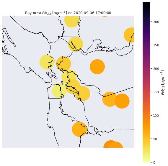
After filtering data to multiple Bay Area cities, now we can see how the PM2.5 concentrations changed over time by animating the static images.
single = vu.pointmap_single(loc_name='Bay Area', param='$PM_{2.5}\;[\mu gm^{-3}]$',data = bay_data, date1=col_list[1], basemap=world, center_lat=37.8711428, center_lon=-122.3714777,
                 color_min=0, color_max=342, xmin=-50000,xmax=60000, ymin=-60000, ymax=50000, min_scale=50, max_scale=50, save=False,save_loc='figures/')
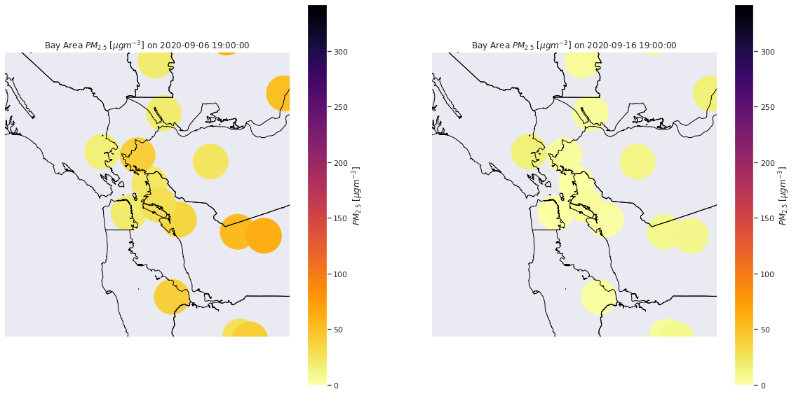
compare = vu.pointmap_compare(bay_data, world, loc_name='Bay Area', param='$PM_{2.5}\;[\mu gm^{-3}]$', date1='2020-09-06 19:00:00', date2='2020-09-16 19:00:00', center_lat=37.8711428, center_lon=-122.3714777,
                 color_min=0, color_max=342, xmin=-50000,xmax=60000, ymin=-60000, ymax=50000, min_scale=50, max_scale=50, save=False, save_loc='figures/')
if animate:
    filenames = []
    j=6
    for i in range(1,12):
        # plot the line chart
        j=5+i
        if j < 10:
            date_to_use = '2020-09-0'+str(j)+' 19:00:00'
        else:
            date_to_use = '2020-09-'+str(j)+' 19:00:00'
        vu.pointmap_single(loc_name='Bay Area', param='$PM_{2.5}\;[\mu gm^{-3}]$',data = bay_data, date1=date_to_use, basemap=world, center_lat=37.8711428, center_lon=-122.3714777,
                 color_min=0, color_max=342, xmin=-50000,xmax=60000, ymin=-60000, ymax=50000, min_scale=50, max_scale=50, save=False,save_loc='figures/')

#         # create file name and append it to a list
        filename = f'figures/animation_frames/simpleframe_{i}.png'
        filenames.append(filename)

#         # save frame
        plt.savefig(filename)
        plt.close()

    with imageio.get_writer('figures/simpletimelapsegif.gif', mode='I', fps=1) as writer:
        for filename in filenames:
            image = imageio.imread(filename)
            writer.append_data(image)

    for filename in set(filenames):
        os.remove(filename)
with open('figures/simpletimelapsegif.gif','rb') as file:
    display(Image(file.read()))
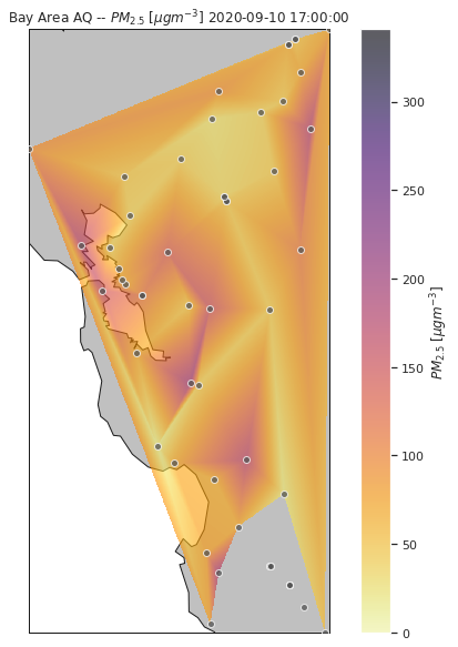
Now lets use a colormesh to linearly interpolate between the points to see how the areas surrounding the Bay Area change over time.
vu.aqviz(dataframe=bay_data, coords=coord_list, region='Bay Area',date='2020-09-10 17:00:00', param='$PM_{2.5}\;[\mu gm^{-3}]$', save=False, save_loc='figures/')
<Figure size 432x288 with 0 Axes>
if animate:
    filenames = []
    for i in range(1,len(col_list)-1):
        # plot the line chart
        vu.aqviz(dataframe=bay_data, coords=coord_list, date=col_list[i], param='$PM_{2.5}\;[\mu gm^{-3}]$', save=False, save_loc='figures/')

#         # create file name and append it to a list
        filename = f'figures/animation_frames/CAframe_{i}.png'
        filenames.append(filename)

#         # save frame
        plt.savefig(filename)
        plt.close()

    with imageio.get_writer('figures/CAtimelapsegif.gif', mode='I') as writer:
        for filename in filenames:
            image = imageio.imread(filename)
            writer.append_data(image)

    for filename in set(filenames):
        os.remove(filename)
with open('figures/timelapsegif.gif','rb') as file:
    display(Image(file.read()))
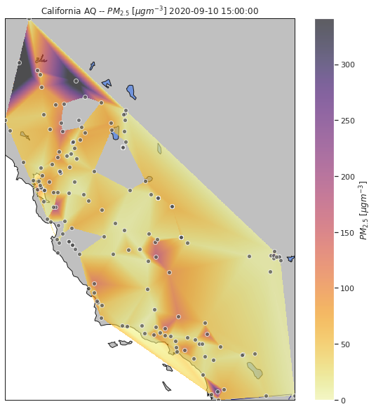
It would be helpful if we could expand this visualization to the rest of California, to see potentially if the particulates in the Bay Area possibly had an impact on other parts of the state, particularly in the days after the second peak when it appeared to dissipate in the Bay Area.
# Commented out so we don't make too many API calls

# filtered_CA_locs = vu.location_filter(USlocs, minlat = 32, minlon = -124, maxlat=42, maxlon = -114, starttime='2020-09-07', endtime='2020-09-17')
# CA_df = vu.param_data_per_loc_for_period(filtered_CA_locs, start_date= '2020-09-07', end_date='2020-09-17', param='pm25', limit=1000, interpolate=True)
# cities_coordinates, coord_list = vu.cities_coords(filtered_CA_locs, CA_df)
# CA_dark_days_data = vu.merge_and_save_gdf(cities_coords=cities_coordinates, data=CA_df, save=True, filename='data/CAdarkdays.geojson')
import json
# with open("data/file.json", 'w') as f:
#     json.dump(coord_list, f, indent=2)

with open("data/file.json", 'r') as f:
    coord_list = json.load(f)
plt.cla()
CA_data = gpd.read_file('data/CAdarkdays.geojson')
col_list = CA_data.columns
vu.aqviz(dataframe=CA_data, coords=coord_list, region = 'California', date=dark_max[0], param='$PM_{2.5}\;[\mu gm^{-3}]$', save=False, save_loc='figures/')
<Figure size 432x288 with 0 Axes>
if animate:
    filenames = []
    for i in range(1,len(col_list)-1):
        # plot the line chart
        vu.aqviz(dataframe=CA_data, coords=coord_list, date=col_list[i], param='$PM_{2.5}\;[\mu gm^{-3}]$', save=False, save_loc='figures/')

#         # create file name and append it to a list
        filename = f'figures/animation_frames/CAframe_{i}.png'
        filenames.append(filename)

#         # save frame
        plt.savefig(filename)
        plt.close()

    with imageio.get_writer('figures/CAtimelapsegif.gif', mode='I') as writer:
        for filename in filenames:
            image = imageio.imread(filename)
            writer.append_data(image)

    for filename in set(filenames):
        os.remove(filename)
with open('figures/CAtimelapsegif.gif','rb') as file:
    display(Image(file.read()))