Demographics in the United States¶

An exploration of the relationships that exist between demographic datapoints¶

Introduction¶

The United States is comprised of so many types of people and jobs, all making different amounts of money with different backgrounds and levels of education. As a country there are many systems in place that limit or guarantee certain future employment opportunities, depending on different qualities like race, gender, and education.

In this report, we explore the relationships between the features in our dataset. We seek to understand the imbalances for gender opportunities by stratifying gender over many factors like job title, income, and more. We also attempt to predict one’s likely income amount (over or under the 50k).

The Data¶

The dataset we used is from Kaggle.com, and includes multiple demographic datapoints about individuals in the United States. The dataset contains the following columns:

Age: continuous variable
Workclass: (categorical) Private, Self-emp-not-inc, Self-emp-inc, Federal-gov, Local-gov, State-gov, Without-pay, Never-worked.
Fnlwgt: continuous variable, amount of people with same set of datapoints in the US
Education: (categorical) Bachelors, Some-college, 11th, HS-grad, Prof-school, Assoc-acdm, Assoc-voc, 9th, 7th-8th, 12th, Masters, 1st-4th, 10th, Doctorate, 5th-6th, Preschool.
Education-num: continuous.
Marital-status: (categorical) Married-civ-spouse, Divorced, Never-married, Separated, Widowed, Married-spouse-absent, Married-AF-spouse.
Occupation: (categorical) Tech-support, Craft-repair, Other-service, Sales, Exec-managerial, Prof-specialty, Handlers-cleaners, Machine-op-inspct, Adm-clerical, Farming-fishing, Transport-moving, Priv-house-serv, Protective-serv, Armed-Forces.
Relationship: (categorical) Wife, Own-child, Husband, Not-in-family, Other-relative, Unmarried.
Race: (categorical) White, Asian-Pac-Islander, Amer-Indian-Eskimo, Other, Black.
Sex: (categorical) Female, Male.
Capital-gain: continuous variable
Capital-loss: continuous variable
Hours-per-week: continuous variable
Native-country: (categorical) United-States, Cambodia, England, Puerto-Rico, Canada, Germany, Outlying-US(Guam-USVI-etc), India, Japan, Greece, South, China, Cuba, Iran, Honduras, Philippines, Italy, Poland, Jamaica, Vietnam, Mexico, Portugal, Ireland, France, Dominican-Republic, Laos, Ecuador, Taiwan, Haiti, Columbia, Hungary, Guatemala, Nicaragua, Scotland, Thailand, Yugoslavia, El-Salvador, Trinadad&Tobago, Peru, Hong, Holand-Netherlands.
Label: (categorical) Over_50k, Under_50k

Package Imports¶

import numpy as np
import seaborn as sns
import pandas as pd
import matplotlib.pyplot as plt
from sklearn.tree import DecisionTreeClassifier
from sklearn.model_selection import train_test_split
from sklearn import metrics
from sklearn import tree
from IPython.display import Image

from gender_functions import plot_gender_eda
from gender_functions import process_df
from gender_functions import plot_tree

Data Import¶

df = pd.read_csv('adult.data', header = None)
df.columns = ['age', 'workclass', 'fnlwgt', 'education', 'education-num', 'marital-status','occupation',
              'relationship', 'race', 'sex','capital-gain','capital-loss','hours-per-week','native country','label']
df.head()

	age	workclass	fnlwgt	education	education-num	marital-status	occupation	relationship	race	sex	capital-gain	hours-per-week	native country	label
0	39	State-gov	77516	Bachelors	13	Never-married	Adm-clerical	Not-in-family	White	Male	2174	40	United-States	<=50K
1	50	Self-emp-not-inc	83311	Bachelors	13	Married-civ-spouse	Exec-managerial	Husband	White	Male	0	13	United-States	<=50K
2	38	Private	215646	HS-grad	9	Divorced	Handlers-cleaners	Not-in-family	White	Male	0	40	United-States	<=50K
3	53	Private	234721	11th	7	Married-civ-spouse	Handlers-cleaners	Husband	Black	Male	0	40	United-States	<=50K
4	28	Private	338409	Bachelors	13	Married-civ-spouse	Prof-specialty	Wife	Black	Female	0	40	Cuba	<=50K

Exploritory Data Analysis¶

Understanding what our data looks like is important. We want to see what the data looks like, are there any empty or unreliable variables, is the dataset sparse. We also want to find any outliers and remove them.

First, we can see that there are no missing values in this data.

df.isnull().sum()

age               0
workclass         0
fnlwgt            0
education         0
education-num     0
marital-status    0
occupation        0
relationship      0
race              0
sex               0
capital-gain      0
capital-loss      0
hours-per-week    0
native country    0
label             0
dtype: int64

Since age is correlated with income, older individulas tend to have higher income due to their experience in the fields. We can see that 43.7% of our data contains Americans over 40 years old.

len(df[df['age'] >= 40]) / len(df)

0.437240870980621

Next, we want to explore the income level of Americans. This dataset found that 24720 individuals make less than 50k a year and 7841 individuals earn more than 50k a year. Therefore, the percentage of Americans that makes more than 50k a year is around 24%.

df.label.value_counts()

 <=50K    24720
 >50K      7841
Name: label, dtype: int64

# Percent of americans making more than 50k a year
7841 / len(df)

0.2408095574460244

We want to see if more Americans over 40 years old make more than 50k a year. Assuming one makes more money as they age, we should see an increase. We found that 9216 individuals earn less than 50k and 5021 individuals who make more than 50k a year over 40 years old. The percentage of Americans over 40 years old and making over 50k a year is 35.3% which is higher than the Americans making over 50k a year without age boundary.

df_over40 = df[df['age'] >= 40]
df_over40.label.value_counts()

 <=50K    9216
 >50K     5021
Name: label, dtype: int64

# Percentage of American over 40 and make more than 50k a year
5021 / len(df_over40)

0.35267261361241836

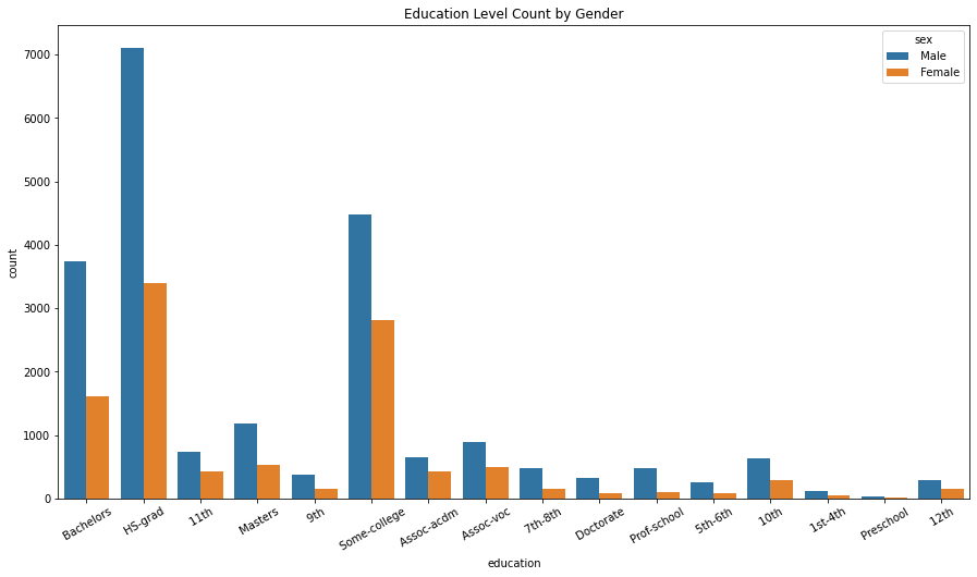
To explore the education level difference in gender, we created a count plot. We found that more males completed the same education level than females such that more males completed bachelor’s than females. The data set contains more males than females. Without specifying the counts, we can see the overall trend that more males completed education than females.

plt.figure(figsize = (15,8))
ax = sns.countplot(x = 'education', hue = 'sex', data = df)
ax.set_xticklabels(ax.get_xticklabels(),rotation = 30)
plt.title('Education Level Count by Gender')
plt.show()

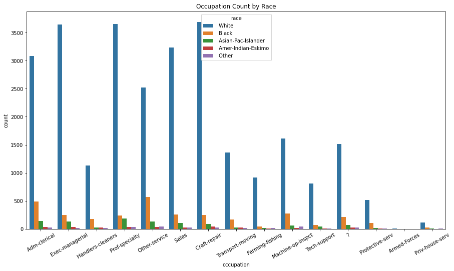
We also want to explore if different races would be more likely to be in a particular occupation. There are more white people in the dataset overthrowing the proportion of the graph, making it unclear to see a trend directly from this plot.

plt.figure(figsize = (15,8))
ax = sns.countplot(x = 'occupation', hue = 'race', data = df)
ax.set_xticklabels(ax.get_xticklabels(),rotation = 30)
plt.title('Occupation Count by Race')
plt.show()

We want to exclude the possible outliers in our data to obtain a more accurate analysis of demographic data points. We exclude the distribution above 99 percent quantile or below the 1 percent quantile limit. This means anyone older than 74 or younger than 17 years old will not be included in the analysis.

def filter_outliers(df, column):
    q_low = df[column].quantile(0.01)
    q_hi  = df[column].quantile(0.99)
    filter_df = df[(df[column] < q_hi) & (df[column] > q_low)]
    return filter_df

df = filter_outliers(df, 'age')
df.head()

	age	workclass	fnlwgt	education	education-num	marital-status	occupation	relationship	race	sex	capital-gain	hours-per-week	native country	label
0	39	State-gov	77516	Bachelors	13	Never-married	Adm-clerical	Not-in-family	White	Male	2174	40	United-States	<=50K
1	50	Self-emp-not-inc	83311	Bachelors	13	Married-civ-spouse	Exec-managerial	Husband	White	Male	0	13	United-States	<=50K
2	38	Private	215646	HS-grad	9	Divorced	Handlers-cleaners	Not-in-family	White	Male	0	40	United-States	<=50K
3	53	Private	234721	11th	7	Married-civ-spouse	Handlers-cleaners	Husband	Black	Male	0	40	United-States	<=50K
4	28	Private	338409	Bachelors	13	Married-civ-spouse	Prof-specialty	Wife	Black	Female	0	40	Cuba	<=50K

Gender Analysis¶

The following section explores the gender differences amongst non-instrinsic qualities like education level, income, occupation, working class, and marital status, to understand if there are any predictive features or noteworthy imbalances. Intrinsic features such as race, age, or nationality will not be considered, as these alone don’t have any logical predictive power of gender, and included in the model would not be valid split points.

We first want to evaulate the ration of men to women in this dataset, to give context to any imbalances seen in the variables.

df['sex'].value_counts()/len(df['sex'])

 Male      0.670835
 Female    0.329165
Name: sex, dtype: float64

We can see that there is about 33/66 split on gender. This is important context to plotting relationships.

plot_gender_eda(df)

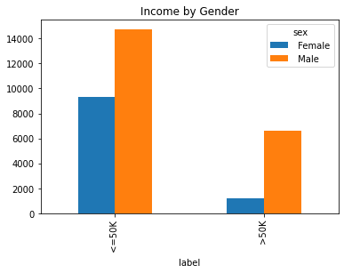
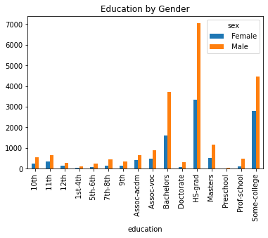
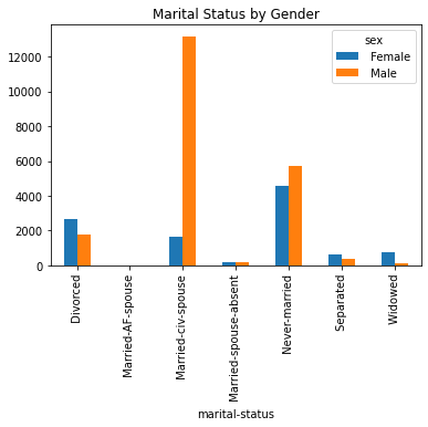
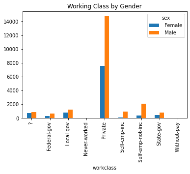
From these plots, we can see there certain variables have more stratification on gender than others. Income, for example, shows that men are more likely to be making >50k. It also shows that men are more likely to be married in this dataset. It also shows that females are more educated.

#Processing our dataframe for our model
X, target = process_df(df, 'sex')
#let's divide our data into a training and testing set, giving our test 15% of the data
X_train, X_test, y_train, y_test = train_test_split(X, target, test_size=0.15, random_state=42)

#using a Decision Tree
clf = DecisionTreeClassifier(max_depth = 3, random_state = 42)
clf = clf.fit(X_train,y_train)
clf.feature_names = list(X_train.columns.values)
y_pred = clf.predict(X_test)

Let’s see how accurate is our model.

metrics.accuracy_score(y_test, y_pred)

0.7275392670157068

The below is a visualization of the decision tree.

plot_tree(clf, target)

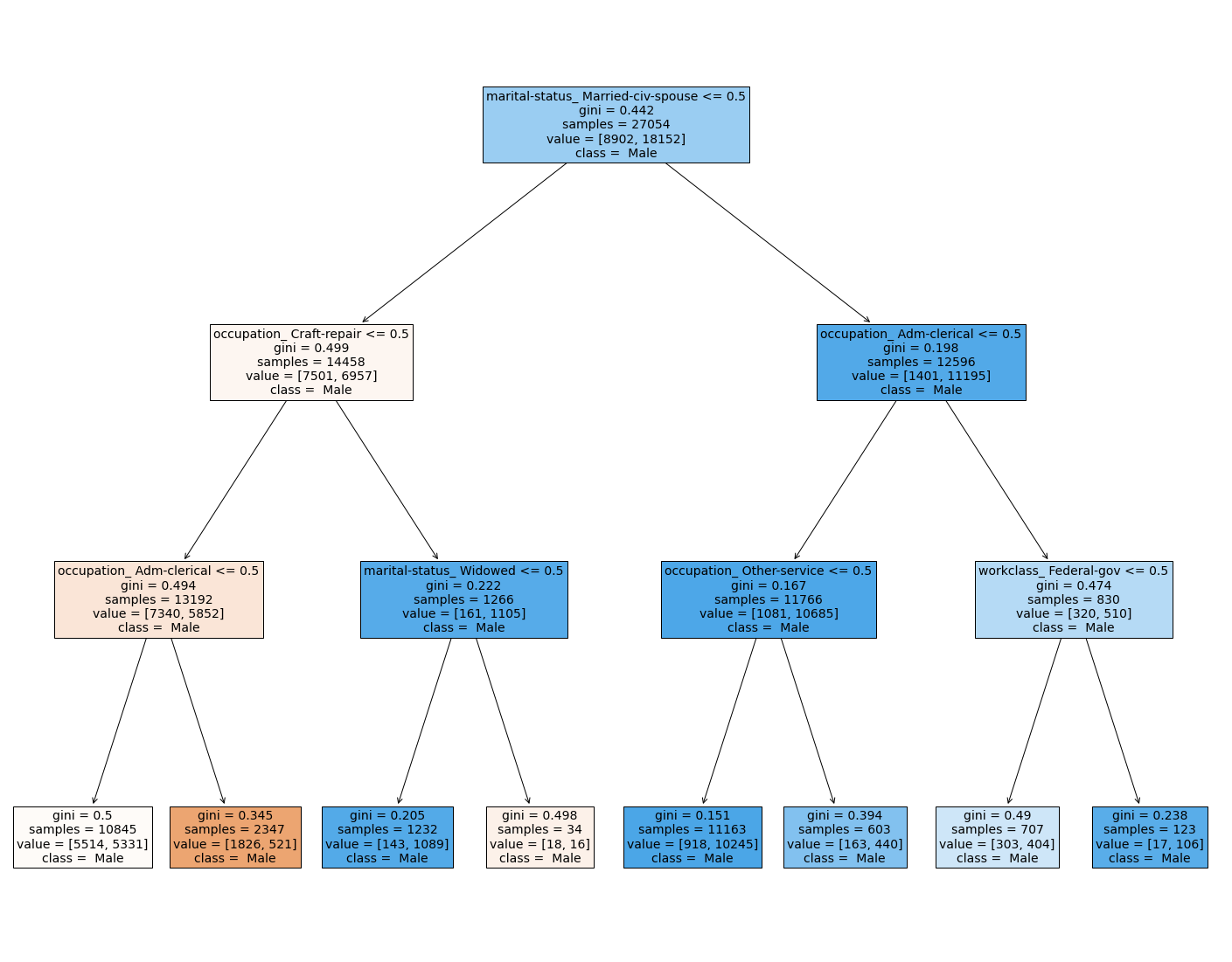
We can see from the decision tree that there is still a lot of impurity in each split, meaning that no single factor is helping to determine gender totally.

Income Prediction¶

The following section explores the predictive power of our features on the income variable. We are using a decision tree model, with an ensemble method for accuracy improvements.

An important contextual cue for this analysis is the dataset’s income ratio of: over 50k and less than (or equal to) 50k

df['label'].value_counts()/len(df['label'])

 <=50K    0.755506
 >50K     0.244494
Name: label, dtype: float64

As we can see, there is a roughly, 24:76 split.

After doing some pre-processing. Including the creation of dummy-variables for all qualitative predictors in the dataset. Five different decision tree models were applied to the dataset to predict income. These models include a naïve, “CART”, decision tree; a bagged decision tree; a bagged decision tree with support-vector-machine feature selection; a bagged decision tree with symmetric-uncertainty feature selection; and, a bagged decision tree with principal component analysis feature selection. These model types vary in complexity, but, a best model could be selected out of them all by using 10-fold cross validation. Please refer to income.ipynb for compuatations involved in these steps.

Image(filename='figures/accuracy_barchart.png')

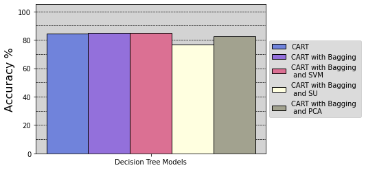
As seen by this barchart- after creating the five, decision tree models. Although only slightly, the best performer- which obtains the highest, 10-fold, cross-validation accuracy. Is the decision tree, with bagging, and support vector machine feature selection. More specifically, its accuracy tends closely towards 85%.

Image(filename='figures/income_tree.png')

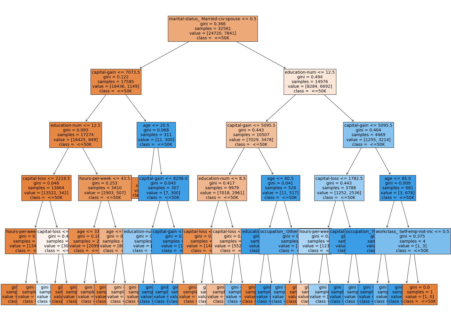
As seen by the above figure, this is what the best model for income prediction looks like. Again, this is the bagged decision tree with support-vector-machine feature selection. Also, please refer to income.ipynb for compuatations involved in these steps.

Results and Limitations¶

From the gender exploration, we can’t conclude too much predictive nature of the features in our dataset. The accuracy of the model was not impressive, and furthermore we can’t assume it was splitting on anything truly predictive. In general however, there is generally a inequal representation of women in many different factors, such as the income gap. Additionally, our dataset may have been an unreliable source in some ways because of the unequal representation of gender in the data.

Overall, with gender, there is data suggesting women may be more educated than men in general, yes overall are less likely to make money.

Now, moving along to our analysis of incomes we have conclude the following. As seen the anaylsis, the best decision tree model is definitely the bagged decision tree with support-vector-machine feature selection. It gives a roughly, 85% accuracy- which in many cases is truly desirable. Nevertheless, despite this accuracy being quite high- it is not great given that the categorical response variable for income is split 76:24. As a result, we have to conclude that decision tree modelling has not been impressive in predicting income levels using the Census Bureau data. At most, it does a slightly better job than prediciting everybody will have a less than 50 thousand dollar income. Perhaps a new dataset, or other modelling method may be more insightful.

The limitations of this dataset come from unrepresentativeness. The categories (race, occupation, native country) in this dataset are not conclusive. The data consists of primarily white males, creating biases in the training models for predictions on both gender analysis and income prediction. The models in this project capture the big picture and ideas that can explore the demographics in the United States. The data only has an income level of over 50k and under 50k. If the data can have numerical values of the actual income instead of a categorical label, it can help to explore more about the income. It would also be beneficial if the data could include geographic locations such as states or cities that can help understand more about each state’s demographic in the United States.

Author Contributions¶

Midori - I created the EDA section before the gender analysis section. I helped with structuring the README file and with making the Jupyter Book.

Samantha - I helped the team create template files for the EDA and Main ipynb files. I completed the gender exploration section, along with the gender_functions package folder and function tests. Helped write the narrative on the main ipynb file. Helped team with git workflow.

Noam - I contributed to the: income decision tree analyses and corresponding write-up, Makefile, environment, readme, jupyter book, and group- Zoom and Slack- discussions.

STAT 159 Group 23 Book

Demographics in the United States

Contents